Support Vector Machine Classifier Implementation in R with caret package

Support Vector Machine Implementation in R Programming Language
Support Vector Machine Classifier implementation in R with the caret package
In the introduction to support vector machine classifier article, we learned about the key aspects as well as the mathematical foundation behind SVM classifier. In this article, we are going to build a Support Vector Machine Classifier using the R programming language. To build the SVM classifier we are going to use the R machine learning caret package.
As we discussed the core concepts behind the SVM algorithm in our previous post it will be a great move to implement the concepts we have learned. If you don’t have the basic understanding of an SVM algorithm, it’s suggested to read our introduction to support vector machines article.
SVM Classifier implementation in R
For SVM classifier implementation in R programming language using caret package, we are going to examine a tidy dataset of Heart Disease. Our motive is to predict whether a patient is having heart disease or not.
To work on big datasets, we can directly use some machine learning packages. The developer community of R programming language has built some great packages to make our work easier. The beauty of these packages is that they are well optimized and can handle maximum exceptions to make our job simple, we just need to call functions for implementing algorithms with the right parameters.
For machine learning, the caret package is a nice package with proper documentation. For Implementing a support vector machine, we can use the caret or e1071 package etc.
The principle behind an SVM classifier (Support Vector Machine) algorithm is to build a hyperplane separating data for different classes. This hyperplane building procedure varies and is the main task of an SVM classifier. The main focus while drawing the hyperplane is on maximizing the distance from hyperplane to the nearest data point of either class. These nearest data points are known as Support Vectors.
Caret Package Installation
The R programming machine learning caret package( Classification And REgression Training ) holds tons of functions that help to build predictive models. It holds tools for data splitting, pre-processing, feature selection, tuning, and supervised – unsupervised learning algorithms, etc. It is similar to sklearn library in python.
For using it, we first need to install it. Open R console and install it by typing:
install.packages(“caret”)
caret package provides us direct access to various functions for training our model with various machine learning algorithms like Knn, SVM, decision tree, linear regression, etc.
Heart Disease Recognition Data Set Description
Heart Disease data set consists of 14 attributes data. All the attributes consist of numeric values. The first 13 variables will be used for predicting 14th variables. The target variable is at index 14.
| Feature Title | Variable Data Type | Feature Categorization | |
| 1. | age | Continuous Variable | 29 – 77 |
| 2. | sex | Categorical Variable | 1 = male; 0 = female |
| 3. | cp: chest pain type | Categorical Variable | 1: typical angina 2: atypical angina 3: non-anginal pain 4: asymptomatic |
| 4. | trestbps: resting blood pressure | Continuous Variable | 94 – 200 |
| 5. | chol: serum cholestoral | Continuous Variable | 126 – 564 |
| 6. | fbs: fasting blood sugar > 120 mg/dl | Categorical Variable | 1 = true; 0 = false |
| 7. | restecg:resting ECG results | Categorical Variable | 0: normal 1: having ST-T wave abnormality |
| 8. | thalach: maximum heart rate achieved | Continuous Variable | 71 – 202 |
| 9. | exang: exercise-induced angina | Categorical Variable | 1 = yes; 0 = no |
| 10. | oldpeak: ST depression induced by exercise relative to rest | Continuous Variable | 0 – 6.2 |
| 11. | slope: slope of the peak exercise ST segment | Continuous Variable | 1 – 3 |
| 12. | ca: number of major vessels | Continuous Variable | 0 – 3 |
| 13. | thal | Categorical Variable | 3 = normal; 6 = fixed defect; 7 = reversible defect |
| 14 | Target Variable | Categorical Variable | 0: Absence of Heart Disease 1: Presence of Heart Disease |
The above table shows all the details of the data.
Heart Disease Recognition Problem Statement
To model a classifier for predicting whether a patient is suffering from any heart disease or not.
SVM classifier implementation in R with Caret Package
R caret Library:
For implementing SVM in r, we only need to import the caret package. As we mentioned above, it helps to perform various tasks to perform our machine learning work. Just past the below command in R console to import r machine learning package Caret.
library(caret)
Data Import
For importing the data and manipulating it, we are going to use data frames. First of all, we need to download the dataset. You can download the dataset our repository. It’s a CSV file i.e, Comma Separated Values file. All the data values are separated by commas. After downloading the CSV file, you need to set your working directory via console else save the data file in your current working directory.
You can get the path of your current working by running the command getwd() in R console. If you wish to change your working directory then follow the below command to get your task completed.
setwd(<PATH of NEW Working Directory>)
Now let’s read the downloaded CSV file into a data frame.
heart_df <- read.csv("heart_tidy.csv", sep = ',', header = FALSE)
For importing data into an R data frame, we can use read.csv() method with parameters as a file name and whether our dataset consists of the 1st row with a header or not. If a header row exists then, the header should be set TRUE else header should set to FALSE.
For checking the structure of data frame we can call the function str() over heart_df:
> str(heart_df)
'data.frame':	300 obs. of  14 variables:
 $ V1 : int  63 67 67 37 41 56 62 57 63 53 ...
 $ V2 : int  1 1 1 1 0 1 0 0 1 1 ...
 $ V3 : int  1 4 4 3 2 2 4 4 4 4 ...
 $ V4 : int  145 160 120 130 130 120 140 120 130 140 ...
 $ V5 : int  233 286 229 250 204 236 268 354 254 203 ...
 $ V6 : int  1 0 0 0 0 0 0 0 0 1 ...
 $ V7 : int  2 2 2 0 2 0 2 0 2 2 ...
 $ V8 : int  150 108 129 187 172 178 160 163 147 155 ...
 $ V9 : int  0 1 1 0 0 0 0 1 0 1 ...
 $ V10: num  2.3 1.5 2.6 3.5 1.4 0.8 3.6 0.6 1.4 3.1 ...
 $ V11: int  3 2 2 3 1 1 3 1 2 3 ...
 $ V12: int  0 3 2 0 0 0 2 0 1 0 ...
 $ V13: int  6 3 7 3 3 3 3 3 7 7 ...
 $ V14: int  0 1 1 0 0 0 1 0 1 1 ...
The above output shows us that our dataset consists of 300 observations each with 14 attributes.
To check top 5-6 rows of the dataset, we can use head().
> head(heart_df)
  V1 V2 V3  V4  V5 V6 V7  V8 V9 V10 V11 V12 V13 V14
1 63  1  1 145 233  1  2 150  0 2.3   3   0   6   0
2 67  1  4 160 286  0  2 108  1 1.5   2   3   3   1
3 67  1  4 120 229  0  2 129  1 2.6   2   2   7   1
4 37  1  3 130 250  0  0 187  0 3.5   3   0   3   0
5 41  0  2 130 204  0  2 172  0 1.4   1   0   3   0
6 56  1  2 120 236  0  0 178  0 0.8   1   0   3   0
The Range of values of the attributes are different but all attributes consist of numeric data.
Data Slicing
Data slicing is a step to split data into train and test set. Training data set can be used specifically for our model building. Test dataset should not be mixed up while building model. Even during standardization, we should not standardize our test set.
set.seed(3033)
intrain <- createDataPartition(y = heart_df$V14, p= 0.7, list = FALSE)
training <- heart_df[intrain,]
testing <- heart_df[-intrain,]
The set.seed() method is used to make our work replicable. As we want our readers to learn concepts by coding these snippets. To make our answers replicable, we need to set a seed value. During partitioning of data, it splits randomly but if our readers will pass the same value in the set.seed() method. Then we both will get identical results.
The caret package provides a method createDataPartition() for partitioning our data into train and test set. We are passing 3 parameters. The “y” parameter takes the value of variable according to which data needs to be partitioned. In our case, target variable is at V14, so we are passing heart_df$V14 (heart data frame’s V14 column).
The “p” parameter holds a decimal value in the range of 0-1. It’s to show that percentage of the split. We are using p=0.7. It means that data split should be done in 70:30 ratio. The “list” parameter is for whether to return a list or matrix. We are passing FALSE for not returning a list. The createDataPartition() method is returning a matrix “intrain” with record’s indices.
By passing values of intrain, we are splitting training data and testing data.
The line training <- heart_df[intrain,] is for putting the data from data frame to training data. Remaining data is saved in the testing data frame, testing <- heart_df[-intrain,].
For checking the dimensions of our training data frame and testing data frame, we can use these.
> dim(training); dim(testing);
[1] 210  14
[1] 90 14
Preprocessing & Training
Preprocessing is all about correcting the problems in data before building a machine learning model using that data. Problems can be of many types like missing values, attributes with a different range, etc.
To check whether our data contains missing values or not, we can use anyNA() method. Here, NA means Not Available.
> anyNA(heart_df)
[1] FALSE
Since it’s returning FALSE, it means we don’t have any missing values.
Dataset summarized details
For checking the summarized details of our data, we can use summary() method. It will give us a basic idea about our dataset’s attributes range.
> summary(heart_df)
       V1              V2             V3              V4              V5
 Min.   :29.00   Min.   :0.00   Min.   :1.000   Min.   : 94.0   Min.   :126.0
 1st Qu.:48.00   1st Qu.:0.00   1st Qu.:3.000   1st Qu.:120.0   1st Qu.:211.0
 Median :56.00   Median :1.00   Median :3.000   Median :130.0   Median :241.5
 Mean   :54.48   Mean   :0.68   Mean   :3.153   Mean   :131.6   Mean   :246.9
 3rd Qu.:61.00   3rd Qu.:1.00   3rd Qu.:4.000   3rd Qu.:140.0   3rd Qu.:275.2
 Max.   :77.00   Max.   :1.00   Max.   :4.000   Max.   :200.0   Max.   :564.0
       V6               V7               V8              V9
 Min.   :0.0000   Min.   :0.0000   Min.   : 71.0   Min.   :0.0000
 1st Qu.:0.0000   1st Qu.:0.0000   1st Qu.:133.8   1st Qu.:0.0000
 Median :0.0000   Median :0.5000   Median :153.0   Median :0.0000
 Mean   :0.1467   Mean   :0.9867   Mean   :149.7   Mean   :0.3267
 3rd Qu.:0.0000   3rd Qu.:2.0000   3rd Qu.:166.0   3rd Qu.:1.0000
 Max.   :1.0000   Max.   :2.0000   Max.   :202.0   Max.   :1.0000
      V10            V11             V12            V13             V14
 Min.   :0.00   Min.   :1.000   Min.   :0.00   Min.   :3.000   Min.   :0.00
 1st Qu.:0.00   1st Qu.:1.000   1st Qu.:0.00   1st Qu.:3.000   1st Qu.:0.00
 Median :0.80   Median :2.000   Median :0.00   Median :3.000   Median :0.00
 Mean   :1.05   Mean   :1.603   Mean   :0.67   Mean   :4.727   Mean   :0.46
 3rd Qu.:1.60   3rd Qu.:2.000   3rd Qu.:1.00   3rd Qu.:7.000   3rd Qu.:1.00
 Max.   :6.20   Max.   :3.000   Max.   :3.00   Max.   :7.000   Max.   :1.00
From above summary statistics, it shows us that all the attributes have a different range. So, we need to standardize our data. We can standardize data using caret’s preProcess() method.
Our target variable consists of 2 values 0, 1. It should be a categorical variable. To convert these to categorical variables, we can convert them to factors.
training[["V14"]] = factor(training[["V14"]])
The above line of code will convert training data frame’s “V14” column to factor variable.
Training the SVM model
Caret package provides train() method for training our data for various algorithms. We just need to pass different parameter values for different algorithms. Before train() method, we will first use trainControl() method. It controls the computational nuances of the train() method.
trctrl <- trainControl(method = "repeatedcv", number = 10, repeats = 3)
set.seed(3233)

svm_Linear <- train(V14 ~., data = training, method = "svmLinear",
                 trControl=trctrl,
                 preProcess = c("center", "scale"),
                 tuneLength = 10)
We are setting 3 parameters of trainControl() method. The “method” parameter holds the details about resampling method. We can set “method” with many values like “boot”, “boot632”, “cv”, “repeatedcv”, “LOOCV”, “LGOCV” etc. For this tutorial, let’s try to use repeatedcv i.e, repeated cross-validation.
The “number” parameter holds the number of resampling iterations. The “repeats ” parameter contains the complete sets of folds to compute for our repeated cross-validation. We are using setting number =10 and repeats =3. This trainControl() methods returns a list. We are going to pass this on our train() method.
Before training our SVM classifier, set.seed().
For training SVM classifier, train() method should be passed with “method” parameter as “svmLinear”. We are passing our target variable V14. The “V14~.” denotes a formula for using all attributes in our classifier and V14 as the target variable. The “trControl” parameter should be passed with results from our trianControl() method. The “preProcess” parameter is for preprocessing our training data.
As discussed earlier for our data, preprocessing is a mandatory task. We are passing 2 values in our “preProcess” parameter “center” & “scale”. These two help for centering and scaling the data. After preProcessing these convert our training data with mean value as approximately “0” and standard deviation as “1”. The “tuneLength” parameter holds an integer value. This is for tuning our algorithm.
Trained SVM model result
You can check the result of our train() method. We are saving its results in a svm_Linear variable.
> svm_Linear
Support Vector Machines with Linear Kernel

210 samples
 13 predictor
  2 classes: '0', '1'

Pre-processing: centered (13), scaled (13)
Resampling: Cross-Validated (10 fold, repeated 3 times)
Summary of sample sizes: 189, 189, 189, 189, 189, 189, ...
Resampling results:

  Accuracy  Kappa
  0.815873  0.62942

Tuning parameter 'C' was held constant at a value of 1
It’s a linear model therefore, it just tested at value “C” =1.
Test Set Prediction
Now, our model is trained with C value as 1. We are ready to predict classes for our test set. We can use predict() method.
> test_pred <- predict(svm_Linear, newdata = testing)
> test_pred
 [1] 0 1 1 1 0 0 1 0 0 1 0 1 0 1 1 1 0 0 1 0 0 0 1 0 0 0 0 1 0 0 0 1 0 0 0 1 1 1 1 1 0 0 1 0
[45] 0 1 0 1 1 1 1 0 1 1 1 0 0 0 0 0 1 0 1 0 0 1 0 0 0 0 0 1 1 0 1 1 0 0 0 1 1 1 1 0 1 0 0 0
[89] 1 0
Levels: 0 1
The caret package provides predict() method for predicting results. We are passing 2 arguments. Its first parameter is our trained model and second parameter “newdata” holds our testing data frame. The predict() method returns a list, we are saving it in a test_pred variable.
How Accurately our model is working?
Using confusion matrix, we can print statistics of our results. It shows that our model accuracy for test set is 86.67%.
> confusionMatrix(test_pred, testing$V14 )
Confusion Matrix and Statistics

          Reference
Prediction  0  1
         0 45  5
         1  7 33

               Accuracy : 0.8667
                 95% CI : (0.7787, 0.9292)
    No Information Rate : 0.5778
    P-Value [Acc > NIR] : 2.884e-09

                  Kappa : 0.7286
 Mcnemar's Test P-Value : 0.7728

            Sensitivity : 0.8654
            Specificity : 0.8684
         Pos Pred Value : 0.9000
         Neg Pred Value : 0.8250
             Prevalence : 0.5778
         Detection Rate : 0.5000
   Detection Prevalence : 0.5556
      Balanced Accuracy : 0.8669

       'Positive' Class : 0
By following the above procedure we can build our svmLinear classifier.
We can also do some customizations for selecting C value(Cost) in Linear classifier. This can be done by inputting values in grid search. The next code snippet will show you, building & tuning of an SVM classifier with different values of C. We are going to put some values of C using expand.grid() into “grid” dataframe. Next step is to use this dataframe for testing our classifier at specific C values. It needs to be put in train() method with tuneGrid parameter.
> grid <- expand.grid(C = c(0,0.01, 0.05, 0.1, 0.25, 0.5, 0.75, 1, 1.25, 1.5, 1.75, 2,5))
> set.seed(3233)
> svm_Linear_Grid <- train(V14 ~., data = training, method = "svmLinear",
trControl=trctrl,
preProcess = c("center", "scale"),
tuneGrid = grid,
tuneLength = 10)
> svm_Linear_Grid
Support Vector Machines with Linear Kernel
210 samples
13 predictor
2 classes: '0', '1'
Pre-processing: centered (13), scaled (13)
Resampling: Cross-Validated (10 fold, repeated 3 times)
Summary of sample sizes: 189, 189, 189, 189, 189, 189, ...
Resampling results across tuning parameters:
C Accuracy Kappa
0.00 NaN NaN
0.01 0.8222222 0.6412577
0.05 0.8285714 0.6540706
0.10 0.8190476 0.6349189
0.25 0.8174603 0.6324448
0.50 0.8126984 0.6232932
0.75 0.8142857 0.6262578
1.00 0.8158730 0.6294200
1.25 0.8158730 0.6294200
1.50 0.8158730 0.6294200
1.75 0.8126984 0.6230572
2.00 0.8126984 0.6230572
5.00 0.8126984 0.6230572
Accuracy was used to select the optimal model using the largest value.
The final value used for the model was C = 0.05.
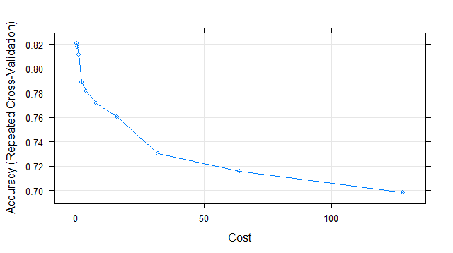
> plot(svm_Linear_Grid)
The above plot is showing that our classifier is giving best accuracy on C = 0.05. Let’s try to make predictions using this model for our test set.
> test_pred_grid <- predict(svm_Linear_Grid, newdata = testing)
> test_pred_grid
 [1] 0 1 1 1 0 0 1 0 0 1 0 1 0 1 1 1 0 0 1 0 0 0 1 0 0 0 0 1 0 0 0 1 0 0 0 1 1 1 1 1 0 0 1 0
[45] 0 1 0 1 1 1 1 0 1 1 1 0 0 0 0 0 0 0 1 0 0 1 0 0 0 0 0 1 1 0 1 1 0 0 0 1 1 1 1 0 1 0 0 0
[89] 1 0
Levels: 0 1
Let’s check its accuracy using confusion -matrix.
> confusionMatrix(test_pred_grid, testing$V14 )
Confusion Matrix and Statistics

          Reference
Prediction  0  1
         0 46  5
         1  6 33

               Accuracy : 0.8778
                 95% CI : (0.7918, 0.9374)
    No Information Rate : 0.5778
    P-Value [Acc > NIR] : 5.854e-10

                  Kappa : 0.7504
 Mcnemar's Test P-Value : 1

            Sensitivity : 0.8846
            Specificity : 0.8684
         Pos Pred Value : 0.9020
         Neg Pred Value : 0.8462
             Prevalence : 0.5778
         Detection Rate : 0.5111
   Detection Prevalence : 0.5667
      Balanced Accuracy : 0.8765

       'Positive' Class : 0
The results of confusion matrix show that this time the accuracy on the test set is 87.78 %.
SVM Classifier using Non-Linear Kernel
In this section, we will try to build a model using Non-Linear Kernel like Radial Basis Function. For using RBF kernel, we just need to change our train() method’s “method” parameter to “svmRadial”. In Radial kernel, it needs to select proper value of Cost “C” parameter and “sigma” parameter.
> set.seed(3233)
> svm_Radial <- train(V14 ~., data = training, method = "svmRadial",
  trControl=trctrl,
  preProcess = c("center", "scale"),
  tuneLength = 10)
> svm_Radial
Support Vector Machines with Radial Basis Function Kernel

210 samples
 13 predictor
  2 classes: '0', '1'

Pre-processing: centered (13), scaled (13)
Resampling: Cross-Validated (10 fold, repeated 3 times)
Summary of sample sizes: 189, 189, 189, 189, 189, 189, ...
Resampling results across tuning parameters:

  C       Accuracy   Kappa
    0.25  0.8206349  0.6380027
    0.50  0.8174603  0.6317534
    1.00  0.8111111  0.6194915
    2.00  0.7888889  0.5750201
    4.00  0.7809524  0.5592617
    8.00  0.7714286  0.5414119
   16.00  0.7603175  0.5202125
   32.00  0.7301587  0.4598166
   64.00  0.7158730  0.4305807
  128.00  0.6984127  0.3966326

Tuning parameter 'sigma' was held constant at a value of 0.04744793
Accuracy was used to select the optimal model using  the largest value.
The final values used for the model were sigma = 0.04744793 and C = 0.25.
> plot(svm_Radial)
It’s showing that final sigma parameter’s value is 0.04744793 & C parameter’s value as 0.25. Let’s try to test our model’s accuracy on our test set. For predicting, we will use predict() with model’s parameters as svm_Radial & newdata= testing.
> test_pred_Radial <- predict(svm_Radial, newdata = testing)
> confusionMatrix(test_pred_Radial, testing$V14 )
Confusion Matrix and Statistics

          Reference
Prediction  0  1
         0 47  6
         1  5 32

               Accuracy : 0.8778
                 95% CI : (0.7918, 0.9374)
    No Information Rate : 0.5778
    P-Value [Acc > NIR] : 5.854e-10

                  Kappa : 0.7486
 Mcnemar's Test P-Value : 1

            Sensitivity : 0.9038
            Specificity : 0.8421
         Pos Pred Value : 0.8868
         Neg Pred Value : 0.8649
             Prevalence : 0.5778
         Detection Rate : 0.5222
   Detection Prevalence : 0.5889
      Balanced Accuracy : 0.8730

       'Positive' Class : 0
We are getting an accuracy of 87.78%. So, in this case with values of C=0.25 & sigma= 0.04744793, we are getting good results.
Let’s try to test & tune our classifier with different values of C & sigma. We will use grid search to implement this.
grid_radial dataframe will hold values of sigma & C. Value of grid_radial will be given to train() method’s tuneGrid parameter.
> grid_radial <- expand.grid(sigma = c(0,0.01, 0.02, 0.025, 0.03, 0.04,
 0.05, 0.06, 0.07,0.08, 0.09, 0.1, 0.25, 0.5, 0.75,0.9),
 C = c(0,0.01, 0.05, 0.1, 0.25, 0.5, 0.75,
 1, 1.5, 2,5))> set.seed(3233)
> svm_Radial_Grid <- train(V14 ~., data = training, method = "svmRadial",
                    trControl=trctrl,
                    preProcess = c("center", "scale"),
                    tuneGrid = grid_radial,
                    tuneLength = 10)

> svm_Radial_Grid
Support Vector Machines with Radial Basis Function Kernel

210 samples
 13 predictor
  2 classes: '0', '1'

Pre-processing: centered (13), scaled (13)
Resampling: Cross-Validated (10 fold, repeated 3 times)
Summary of sample sizes: 189, 189, 189, 189, 189, 189, ...
Resampling results across tuning parameters:

  sigma  C     Accuracy   Kappa
  0.000  0.00        NaN          NaN
  0.000  0.01  0.5238095  0.000000000
  0.000  0.05  0.5238095  0.000000000
  0.000  0.10  0.5238095  0.000000000
  0.000  0.25  0.5238095  0.000000000
  0.000  0.50  0.5238095  0.000000000
  0.000  0.75  0.5238095  0.000000000
  0.000  1.00  0.5238095  0.000000000
  0.000  1.50  0.5238095  0.000000000
  0.000  2.00  0.5238095  0.000000000
  0.000  5.00  0.5238095  0.000000000
  0.010  0.00        NaN          NaN
  0.010  0.01  0.5238095  0.000000000
  0.010  0.05  0.5238095  0.000000000
  0.010  0.10  0.7857143  0.563592267
  0.010  0.25  0.8222222  0.640049451
  0.010  0.50  0.8222222  0.641110091
  0.010  0.75  0.8222222  0.641137925
  0.010  1.00  0.8222222  0.641136734
  0.010  1.50  0.8206349  0.637911063
  0.010  2.00  0.8206349  0.637911063
  0.010  5.00  0.8158730  0.628496247
  0.020  0.00        NaN          NaN
  0.020  0.01  0.5238095  0.000000000
  0.020  0.05  0.6984127  0.377124781
  0.020  0.10  0.8222222  0.639785597
  0.020  0.25  0.8222222  0.640905610
  0.020  0.50  0.8222222  0.641137925
  0.020  0.75  0.8222222  0.641020628
  0.020  1.00  0.8238095  0.644274433
  0.020  1.50  0.8174603  0.631778489
  0.020  2.00  0.8158730  0.628872638
  0.020  5.00  0.7936508  0.584875363
  0.025  0.00        NaN          NaN
  0.025  0.01  0.5238095  0.000000000
  0.025  0.05  0.7523810  0.491454156
  0.025  0.10  0.8222222  0.639930758
  0.025  0.25  0.8206349  0.637798181
  0.025  0.50  0.8206349  0.637882929
  0.025  0.75  0.8222222  0.641020628
  0.025  1.00  0.8253968  0.647704077
  0.025  1.50  0.8142857  0.625619612
  0.025  2.00  0.8111111  0.619606847
  0.025  5.00  0.7873016  0.571968346
  0.030  0.00        NaN          NaN
  0.030  0.01  0.5238095  0.000000000
  0.030  0.05  0.7682540  0.525466210
  0.030  0.10  0.8206349  0.637002421
  0.030  0.25  0.8190476  0.634747262
  0.030  0.50  0.8222222  0.641020628
  0.030  0.75  0.8206349  0.637999463
  0.030  1.00  0.8158730  0.628700648
  0.030  1.50  0.8142857  0.625854896
  0.030  2.00  0.8079365  0.613267389
  0.030  5.00  0.7888889  0.575045900
  0.040  0.00        NaN          NaN
  0.040  0.01  0.5238095  0.000000000
  0.040  0.05  0.7825397  0.555882207
  0.040  0.10  0.8238095  0.643780156
  0.040  0.25  0.8174603  0.631462266
  0.040  0.50  0.8190476  0.634861764
  0.040  0.75  0.8174603  0.631866717
  0.040  1.00  0.8174603  0.632128942
  0.040  1.50  0.8063492  0.610017781
  0.040  2.00  0.7936508  0.584994041
  0.040  5.00  0.7793651  0.556410718
  0.050  0.00        NaN          NaN
  0.050  0.01  0.5238095  0.000000000
  0.050  0.05  0.7746032  0.539572451
  0.050  0.10  0.8222222  0.640843896
  0.050  0.25  0.8206349  0.638002663
  0.050  0.50  0.8174603  0.631665417
  0.050  0.75  0.8158730  0.628641594
  0.050  1.00  0.8095238  0.616296629
  0.050  1.50  0.7936508  0.585141338
  0.050  2.00  0.7904762  0.578416665
  0.050  5.00  0.7746032  0.546944215
  0.060  0.00        NaN          NaN
  0.060  0.01  0.5238095  0.000000000
  0.060  0.05  0.7539683  0.495857444
  0.060  0.10  0.8222222  0.640843896
  0.060  0.25  0.8174603  0.631610502
  0.060  0.50  0.8111111  0.619201644
  0.060  0.75  0.8095238  0.616267035
  0.060  1.00  0.8031746  0.603625492
  0.060  1.50  0.7873016  0.572031467
  0.060  2.00  0.7968254  0.591535559
  0.060  5.00  0.7793651  0.556715449
  0.070  0.00        NaN          NaN
  0.070  0.01  0.5238095  0.000000000
  0.070  0.05  0.7396825  0.465403075
  0.070  0.10  0.8222222  0.640784261
  0.070  0.25  0.8158730  0.628501328
  0.070  0.50  0.8079365  0.612927598
  0.070  0.75  0.8047619  0.607028961
  0.070  1.00  0.7920635  0.581705463
  0.070  1.50  0.7904762  0.578630216
  0.070  2.00  0.7952381  0.588103221
  0.070  5.00  0.7793651  0.557723627
  0.080  0.00        NaN          NaN
  0.080  0.01  0.5238095  0.000000000
  0.080  0.05  0.7142857  0.411697289
  0.080  0.10  0.8206349  0.637529265
  0.080  0.25  0.8095238  0.616007758
  0.080  0.50  0.8079365  0.613071572
  0.080  0.75  0.7984127  0.594146715
  0.080  1.00  0.7904762  0.578715332
  0.080  1.50  0.7984127  0.594647071
  0.080  2.00  0.7904762  0.578689209
  0.080  5.00  0.7777778  0.554522065
  0.090  0.00        NaN          NaN
  0.090  0.01  0.5238095  0.000000000
  0.090  0.05  0.6634921  0.303570375
  0.090  0.10  0.8222222  0.640490820
  0.090  0.25  0.8079365  0.613539156
  0.090  0.50  0.8047619  0.606555347
  0.090  0.75  0.7936508  0.585021621
  0.090  1.00  0.7857143  0.569156095
  0.090  1.50  0.7952381  0.588371141
  0.090  2.00  0.7841270  0.565873887
  0.090  5.00  0.7714286  0.541592623
  0.100  0.00        NaN          NaN
  0.100  0.01  0.5238095  0.000000000
  0.100  0.05  0.6126984  0.194097781
  0.100  0.10  0.8126984  0.620930145
  0.100  0.25  0.8031746  0.604558785
  0.100  0.50  0.8031746  0.603653188
  0.100  0.75  0.7936508  0.584991621
  0.100  1.00  0.7873016  0.572324436
  0.100  1.50  0.7888889  0.575436285
  0.100  2.00  0.7825397  0.562906611
  0.100  5.00  0.7666667  0.531862324
  0.250  0.00        NaN          NaN
  0.250  0.01  0.5238095  0.000000000
  0.250  0.05  0.5238095  0.000000000
  0.250  0.10  0.5238095  0.000000000
  0.250  0.25  0.7428571  0.475302551
  0.250  0.50  0.7666667  0.534771105
  0.250  0.75  0.7539683  0.508759153
  0.250  1.00  0.7603175  0.520171909
  0.250  1.50  0.7444444  0.488760478
  0.250  2.00  0.7460317  0.491872751
  0.250  5.00  0.7412698  0.482972131
  0.500  0.00        NaN          NaN
  0.500  0.01  0.5238095  0.000000000
  0.500  0.05  0.5238095  0.000000000
  0.500  0.10  0.5238095  0.000000000
  0.500  0.25  0.5238095  0.000000000
  0.500  0.50  0.5682540  0.098329296
  0.500  0.75  0.6587302  0.299577029
  0.500  1.00  0.7063492  0.414760542
  0.500  1.50  0.7000000  0.402294266
  0.500  2.00  0.7047619  0.412014316
  0.500  5.00  0.7047619  0.412014316
  0.750  0.00        NaN          NaN
  0.750  0.01  0.5238095  0.000000000
  0.750  0.05  0.5238095  0.000000000
  0.750  0.10  0.5238095  0.000000000
  0.750  0.25  0.5238095  0.000000000
  0.750  0.50  0.5269841  0.006951027
  0.750  0.75  0.5571429  0.074479136
  0.750  1.00  0.6015873  0.179522487
  0.750  1.50  0.6158730  0.213036862
  0.750  2.00  0.6174603  0.217499695
  0.750  5.00  0.6158730  0.214090454
  0.900  0.00        NaN          NaN
  0.900  0.01  0.5238095  0.000000000
  0.900  0.05  0.5238095  0.000000000
  0.900  0.10  0.5238095  0.000000000
  0.900  0.25  0.5238095  0.000000000
  0.900  0.50  0.5238095  0.000000000
  0.900  0.75  0.5444444  0.045715223
  0.900  1.00  0.5444444  0.055590646
  0.900  1.50  0.5698413  0.111517087
  0.900  2.00  0.5698413  0.111517087
  0.900  5.00  0.5698413  0.111517087

Accuracy was used to select the optimal model using  the largest value.
The final values used for the model were sigma = 0.025 and C = 1.

>plot(svm_Radial_Grid)
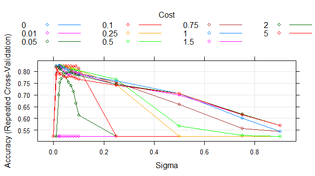
Awesome, we ran our SVM-RBF kernel. It calculated variations and gave us best values of sigma & C. It’s telling us that best values of sigma= 0.025 & C=1 Let’s check our trained models’ accuracy on the test set.
> test_pred_Radial_Grid <- predict(svm_Radial_Grid, newdata = testing)
>
> confusionMatrix(test_pred_Radial_Grid, testing$V14 )
Confusion Matrix and Statistics

          Reference
Prediction  0  1
         0 46  6
         1  6 32

               Accuracy : 0.8667
                 95% CI : (0.7787, 0.9292)
    No Information Rate : 0.5778
    P-Value [Acc > NIR] : 2.884e-09

                  Kappa : 0.7267
 Mcnemar's Test P-Value : 1

            Sensitivity : 0.8846
            Specificity : 0.8421
         Pos Pred Value : 0.8846
         Neg Pred Value : 0.8421
             Prevalence : 0.5778
         Detection Rate : 0.5111
   Detection Prevalence : 0.5778
      Balanced Accuracy : 0.8634

       'Positive' Class : 0
For our svm_Radial_Grid classifier, it’s giving an accuracy of 86.67%. So, it shows Radial classifier is not giving better results as compared to Linear classifier even after tuning it. It may be due to overfitting.
Follow us:
FACEBOOK| QUORA |TWITTER| GOOGLE+ | LINKEDIN| REDDIT | FLIPBOARD | MEDIUM | GITHUB
I hope you like this post. If you have any questions, then feel free to comment below. If you want me to write on one particular topic, then do tell it to me in the comments below.
Related Courses:
Do check out unlimited data science courses
| Title & links | Details | What You Will Learn |
| Machine Learning A-Z: Hands-On Python & R In Data Science
|
Course Overall Rating:: 4.6 |
|
| R Programming A-Z: R For Data Science With Real Exercises!
|
Course Overall Rating:: 4.6 |
|
| Data Mining with R: Go from Beginner to Advanced! |
Course Overall Rating:: 4.2 |
|


svm_Linear <- train(gene ~., data = training, method = "svmLinear",
trControl=trctrl,
preProcess = c("center", "scale"),
tuneLength = 2)
Hi when i used it, warning appears that i am doing regression instead of classification what should I do for classification?
Yes
Great tutorial. For the first model evaluation: confusionMatrix(test_pred, testing$V14), the testing set target variable have to be converted to factor too.
Hi Leke,
Thanks for the compliment.
We wish you a very happy learning.
Would you be able to plot the hyper plane using this? Thanks
Hi Rosie,
We can’t plot the hyperplane with this level of where if we the coefficient of the hyperplane we can easily visualize then using matplotlib or any other visualization package.
Thanks and happy learning!
Thanks for the tutorial! I was wondering what other kernel functions we can use instead of Radial? Thanks again
Hi Rosie,
Below are a few examples for support vector kernels to try out.
Thanks and happy learning!
Hi, is there a way to retrieve the coefficients computed by the SVM model? I’ve built out the model, but am having a hard time to retrieve the coefficients of each predictor. Thank you!
Hi Eleanor,
You can retrieve the build SVM model coefficients with this method svm.coef_ same as the way we get coefficients in linear regression.
Thanks and happy learning!
Hello,
Is this One to One or One to All?
Hi,
I am not sure about the question, Could you please explain it with more context.
Thanks!
Hey for some reason the [intrain, ] function doesn’t work on my R, it can’t find it as an object.
Hi Johan,
Could you check the usage of the function once?
This is Rahul, here your data have 13 dependent variables and how come you know that all these variables are relevant for this model. Is feature selection is very important step before svm? Could you post a topic on feature selection, feature ranking importance and how can we do it in r studio.
Hi Rahul,
Yes, You said correct (y). The main challenging task is feature selection when it’s Machine learning model building. We will try to write an article about the importance of features selections and how to implement feature selection in both python and R.