Support vector machine (Svm classifier) implemenation in python with Scikit-learn


Iris Classification with Svm Classifier
Svm classifier implementation in python with scikit-learn
Support vector machine classifier is one of the most popular machine learning classification algorithm. Svm classifier mostly used in addressing multi-classification problems. If you are not aware of the multi-classification problem below are examples of multi-classification problems.
Multi-Classification Problem Examples:
- Given fruit features like color, size, taste, weight, shape. Predicting the fruit type.
- By analyzing the skin, predicting the different skin disease.
- Given Google news articles, predicting the topic of the article. This could be sport, movie, tech news related article, etc.
In short: Multi-classification problem means having more that 2 target classes to predict.
In the first example of predicting the fruit type. The target class will have many fruits like apple, mango, orange, banana, etc. This is same with the other two examples in predicting. The problem of the new article, the target class having different topics like sport, movie, tech news ..etc
In this article, we were going to implement the svm classifier with different kernels. However, we have explained the key aspect of support vector machine algorithm as well we had implemented svm classifier in R programming language in our earlier posts. If you are reading this post for the first time, it’s recommended to chek out the previous post on svm concepts.
To implement svm classifier in Python, we are going to use the one of most popular classification dataset which is Iris dataset. Let’s quickly look at the features and the target variable details of the famous classification dataset.
Iris Dataset description
Irises dataset for classification
This famous classification dataset first time used in Fisher’s classic 1936 paper, The Use of Multiple Measurements in Taxonomic Problems. Iris dataset is having 4 features of iris flower and one target class.
The 4 features are
- SepalLengthCm
- SepalWidthCm
- PetalLengthCm
- PetalWidthCm
The target class
The flower species type is the target class and it having 3 types
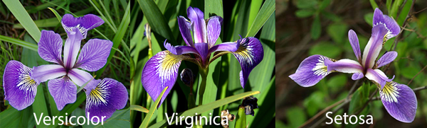
- Setosa
- Versicolor
- Virginica
The idea of implementing svm classifier in Python is to use the iris features to train an svm classifier and use the trained svm model to predict the Iris species type. To begin with let’s try to load the Iris dataset. We are going to use the iris data from Scikit-Learn package.
Analyzing Iris dataset
To successfully run the below scripts in your machine you need to install the required packages. It’s better to please go through the python machine learning packages installation or machine learning packages step up before running the below scripts.
Importing Iris dataset from Scikit-Learn
Let’s first import the required python packages
# Required Packages
from sklearn import datasets		# To Get iris dataset
from sklearn import svm    			# To fit the svm classifier
import numpy as np
import matplotlib.pyplot as plt            # To visuvalizing the data
Now let’s import the iris dataset
# import iris data to model Svm classifier
iris_dataset = datasets.load_iris()
Using the DESCR key over the iris_dataset, we can get description of the dataset
print "Iris data set Description :: ", iris_dataset['DESCR']
Output
Iris data set Description ::  Iris Plants Database

Notes
-----
Data Set Characteristics:
    :Number of Instances: 150 (50 in each of three classes)
    :Number of Attributes: 4 numeric, predictive attributes and the class
    :Attribute Information:
        - sepal length in cm
        - sepal width in cm
        - petal length in cm
        - petal width in cm
        - class:
                - Iris-Setosa
                - Iris-Versicolour
                - Iris-Virginica
    :Summary Statistics:

    ============== ==== ==== ======= ===== ====================
                    Min  Max   Mean    SD   Class Correlation
    ============== ==== ==== ======= ===== ====================
    sepal length:   4.3  7.9   5.84   0.83    0.7826
    sepal width:    2.0  4.4   3.05   0.43   -0.4194
    petal length:   1.0  6.9   3.76   1.76    0.9490  (high!)
    petal width:    0.1  2.5   1.20  0.76     0.9565  (high!)
    ============== ==== ==== ======= ===== ====================

    :Missing Attribute Values: None
    :Class Distribution: 33.3% for each of 3 classes.
    :Creator: R.A. Fisher
    :Donor: Michael Marshall (MARSHALL%PLU@io.arc.nasa.gov)
    :Date: July, 1988

This is a copy of UCI ML iris datasets.
http://archive.ics.uci.edu/ml/datasets/Iris

The famous Iris database, first used by Sir R.A Fisher

This is perhaps the best known database to be found in the
pattern recognition literature.  Fisher's paper is a classic in the field and
is referenced frequently to this day.  (See Duda & Hart, for example.)  The
data set contains 3 classes of 50 instances each, where each class refers to a
type of iris plant.  One class is linearly separable from the other 2; the
latter are NOT linearly separable from each other.

References
----------
   - Fisher,R.A. "The use of multiple measurements in taxonomic problems"
     Annual Eugenics, 7, Part II, 179-188 (1936); also in "Contributions to
     Mathematical Statistics" (John Wiley, NY, 1950).
   - Duda,R.O., & Hart,P.E. (1973) Pattern Classification and Scene Analysis.
     (Q327.D83) John Wiley & Sons.  ISBN 0-471-22361-1.  See page 218.
   - Dasarathy, B.V. (1980) "Nosing Around the Neighborhood: A New System
     Structure and Classification Rule for Recognition in Partially Exposed
     Environments".  IEEE Transactions on Pattern Analysis and Machine
     Intelligence, Vol. PAMI-2, No. 1, 67-71.
   - Gates, G.W. (1972) "The Reduced Nearest Neighbor Rule".  IEEE Transactions
     on Information Theory, May 1972, 431-433.
   - See also: 1988 MLC Proceedings, 54-64.  Cheeseman et al"s AUTOCLASS II
     conceptual clustering system finds 3 classes in the data.
   - Many, many more ...
Now let’s get the iris features and the target classes
print "Iris feature data :: ", iris_dataset['data']
Output
Iris feature data ::  [[ 5.1  3.5  1.4  0.2]
 [ 4.9  3.   1.4  0.2]
 [ 4.7  3.2  1.3  0.2]
 [ 4.6  3.1  1.5  0.2]
 [ 5.   3.6  1.4  0.2]
 [ 5.4  3.9  1.7  0.4]
 [ 4.6  3.4  1.4  0.3]
 [ 5.   3.4  1.5  0.2]
 [ 4.4  2.9  1.4  0.2]
 [ 4.9  3.1  1.5  0.1]
 [ 5.4  3.7  1.5  0.2]
 [ 4.8  3.4  1.6  0.2]
 [ 4.8  3.   1.4  0.1]
 [ 4.3  3.   1.1  0.1]
 [ 5.8  4.   1.2  0.2]
 [ 5.7  4.4  1.5  0.4]
 [ 5.4  3.9  1.3  0.4]
 [ 5.1  3.5  1.4  0.3]
 [ 5.7  3.8  1.7  0.3]
 [ 5.1  3.8  1.5  0.3]
 [ 5.4  3.4  1.7  0.2]
 [ 5.1  3.7  1.5  0.4]
 [ 4.6  3.6  1.   0.2]
 [ 5.1  3.3  1.7  0.5]
 [ 4.8  3.4  1.9  0.2]
 [ 5.   3.   1.6  0.2]
 [ 5.   3.4  1.6  0.4]
 [ 5.2  3.5  1.5  0.2]
 [ 5.2  3.4  1.4  0.2]
 [ 4.7  3.2  1.6  0.2]
 [ 4.8  3.1  1.6  0.2]
 [ 5.4  3.4  1.5  0.4]
 [ 5.2  4.1  1.5  0.1]
 [ 5.5  4.2  1.4  0.2]
 [ 4.9  3.1  1.5  0.1]
 [ 5.   3.2  1.2  0.2]
 [ 5.5  3.5  1.3  0.2]
 [ 4.9  3.1  1.5  0.1]
 [ 4.4  3.   1.3  0.2]
 [ 5.1  3.4  1.5  0.2]
 [ 5.   3.5  1.3  0.3]
 [ 4.5  2.3  1.3  0.3]
 [ 4.4  3.2  1.3  0.2]
 [ 5.   3.5  1.6  0.6]
 [ 5.1  3.8  1.9  0.4]
 [ 4.8  3.   1.4  0.3]
 [ 5.1  3.8  1.6  0.2]
 [ 4.6  3.2  1.4  0.2]
 [ 5.3  3.7  1.5  0.2]
 [ 5.   3.3  1.4  0.2]
 [ 7.   3.2  4.7  1.4]
 [ 6.4  3.2  4.5  1.5]
 [ 6.9  3.1  4.9  1.5]
 [ 5.5  2.3  4.   1.3]
 [ 6.5  2.8  4.6  1.5]
 [ 5.7  2.8  4.5  1.3]
 [ 6.3  3.3  4.7  1.6]
 [ 4.9  2.4  3.3  1. ]
 [ 6.6  2.9  4.6  1.3]
 [ 5.2  2.7  3.9  1.4]
 [ 5.   2.   3.5  1. ]
 [ 5.9  3.   4.2  1.5]
 [ 6.   2.2  4.   1. ]
 [ 6.1  2.9  4.7  1.4]
 [ 5.6  2.9  3.6  1.3]
 [ 6.7  3.1  4.4  1.4]
 [ 5.6  3.   4.5  1.5]
 [ 5.8  2.7  4.1  1. ]
 [ 6.2  2.2  4.5  1.5]
 [ 5.6  2.5  3.9  1.1]
 [ 5.9  3.2  4.8  1.8]
 [ 6.1  2.8  4.   1.3]
 [ 6.3  2.5  4.9  1.5]
 [ 6.1  2.8  4.7  1.2]
 [ 6.4  2.9  4.3  1.3]
 [ 6.6  3.   4.4  1.4]
 [ 6.8  2.8  4.8  1.4]
 [ 6.7  3.   5.   1.7]
 [ 6.   2.9  4.5  1.5]
 [ 5.7  2.6  3.5  1. ]
 [ 5.5  2.4  3.8  1.1]
 [ 5.5  2.4  3.7  1. ]
 [ 5.8  2.7  3.9  1.2]
 [ 6.   2.7  5.1  1.6]
 [ 5.4  3.   4.5  1.5]
 [ 6.   3.4  4.5  1.6]
 [ 6.7  3.1  4.7  1.5]
 [ 6.3  2.3  4.4  1.3]
 [ 5.6  3.   4.1  1.3]
 [ 5.5  2.5  4.   1.3]
 [ 5.5  2.6  4.4  1.2]
 [ 6.1  3.   4.6  1.4]
 [ 5.8  2.6  4.   1.2]
 [ 5.   2.3  3.3  1. ]
 [ 5.6  2.7  4.2  1.3]
 [ 5.7  3.   4.2  1.2]
 [ 5.7  2.9  4.2  1.3]
 [ 6.2  2.9  4.3  1.3]
 [ 5.1  2.5  3.   1.1]
 [ 5.7  2.8  4.1  1.3]
 [ 6.3  3.3  6.   2.5]
 [ 5.8  2.7  5.1  1.9]
 [ 7.1  3.   5.9  2.1]
 [ 6.3  2.9  5.6  1.8]
 [ 6.5  3.   5.8  2.2]
 [ 7.6  3.   6.6  2.1]
 [ 4.9  2.5  4.5  1.7]
 [ 7.3  2.9  6.3  1.8]
 [ 6.7  2.5  5.8  1.8]
 [ 7.2  3.6  6.1  2.5]
 [ 6.5  3.2  5.1  2. ]
 [ 6.4  2.7  5.3  1.9]
 [ 6.8  3.   5.5  2.1]
 [ 5.7  2.5  5.   2. ]
 [ 5.8  2.8  5.1  2.4]
 [ 6.4  3.2  5.3  2.3]
 [ 6.5  3.   5.5  1.8]
 [ 7.7  3.8  6.7  2.2]
 [ 7.7  2.6  6.9  2.3]
 [ 6.   2.2  5.   1.5]
 [ 6.9  3.2  5.7  2.3]
 [ 5.6  2.8  4.9  2. ]
 [ 7.7  2.8  6.7  2. ]
 [ 6.3  2.7  4.9  1.8]
 [ 6.7  3.3  5.7  2.1]
 [ 7.2  3.2  6.   1.8]
 [ 6.2  2.8  4.8  1.8]
 [ 6.1  3.   4.9  1.8]
 [ 6.4  2.8  5.6  2.1]
 [ 7.2  3.   5.8  1.6]
 [ 7.4  2.8  6.1  1.9]
 [ 7.9  3.8  6.4  2. ]
 [ 6.4  2.8  5.6  2.2]
 [ 6.3  2.8  5.1  1.5]
 [ 6.1  2.6  5.6  1.4]
 [ 7.7  3.   6.1  2.3]
 [ 6.3  3.4  5.6  2.4]
 [ 6.4  3.1  5.5  1.8]
 [ 6.   3.   4.8  1.8]
 [ 6.9  3.1  5.4  2.1]
 [ 6.7  3.1  5.6  2.4]
 [ 6.9  3.1  5.1  2.3]
 [ 5.8  2.7  5.1  1.9]
 [ 6.8  3.2  5.9  2.3]
 [ 6.7  3.3  5.7  2.5]
 [ 6.7  3.   5.2  2.3]
 [ 6.3  2.5  5.   1.9]
 [ 6.5  3.   5.2  2. ]
 [ 6.2  3.4  5.4  2.3]
 [ 5.9  3.   5.1  1.8]]
As we are said, these are 4 features first 2 were sepal length, sepal width and the next 2 were petal length and width. Now let’s check the target data
print "Iris target :: ", iris_dataset['target']
Output
Iris target ::  [0 0 0 0 0 0 0 0 0 0 0 0 0 0 0 0 0 0 0 0 0 0 0 0 0 0 0 0 0 0 0 0 0 0 0 0 0
 0 0 0 0 0 0 0 0 0 0 0 0 0 1 1 1 1 1 1 1 1 1 1 1 1 1 1 1 1 1 1 1 1 1 1 1 1
 1 1 1 1 1 1 1 1 1 1 1 1 1 1 1 1 1 1 1 1 1 1 1 1 1 1 2 2 2 2 2 2 2 2 2 2 2
 2 2 2 2 2 2 2 2 2 2 2 2 2 2 2 2 2 2 2 2 2 2 2 2 2 2 2 2 2 2 2 2 2 2 2 2 2
 2 2]
Visualizing the Iris dataset
Let’s take the individual features like sepal, petal length, and weight and let’s visualize the corresponding target classes with different colors.
Visualizing the relationship between sepal and target classes
def visuvalize_sepal_data():
	iris = datasets.load_iris()
	X = iris.data[:, :2]  # we only take the first two features.
	y = iris.target
	plt.scatter(X[:, 0], X[:, 1], c=y, cmap=plt.cm.coolwarm)
	plt.xlabel('Sepal length')
	plt.ylabel('Sepal width')
	plt.title('Sepal Width & Length')
	plt.show()

visuvalize_sepal_data()
To visualize the Sepal length, width and corresponding target classes we can create a function with name visuvalize_sepal_data. At the beginning, we are loading the iris dataset to iris variable. Next, we are storing the first 2 features in iris dataset which are sepal length and sepal width to variable x. Then we are storing the corresponding target values in variable y.
As we have seen target variable contains values like 0, 1,2 each value represents the iris flower species type. Then we are plotting the points on XY axis on X-axis we are plotting Sepal Length values. On Y-axis we are plotting Sepal Width values. If you follow installing instruction correctly on Installing Python machine learning packages and run the above code, you will get the below image.
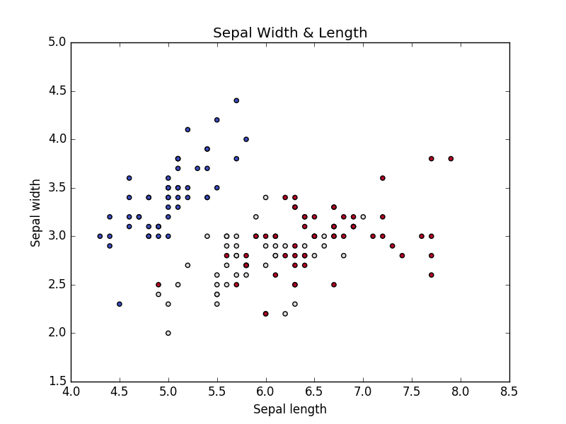
Iris Sepal length & width Vs Iris Species type
Let’s create the similar kind of graph for Petal length and width
Visualizing the relationship between Petal and target classes
def visuvalize_petal_data():
	iris = datasets.load_iris()
	X = iris.data[:, 2:]  # we only take the last two features.
	y = iris.target
	plt.scatter(X[:, 0], X[:, 1], c=y, cmap=plt.cm.coolwarm)
	plt.xlabel('Petal length')
	plt.ylabel('Petal width')
	plt.title('Petal Width & Length')
	plt.show()

visuvalize_petal_data()
If we run the above code, we will get the below graph.
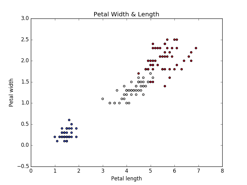
Iris Petal length & width Vs Species Type
As we have successfully visualized the behavior of target class (iris species type) with respect to Sepal length and width as well as with respect to Petal length and width. Now let’s model different kernel Svm classifier by considering only the Sepal features (Length and Width) and only the Petal features (Lenght and Width)
Modeling Different Kernel Svm classifier using Iris Sepal features
iris = datasets.load_iris()
X = iris.data[:, :2]  # we only take the Sepal two features.
y = iris.target
C = 1.0  # SVM regularization parameter

# SVC with linear kernel
svc = svm.SVC(kernel='linear', C=C).fit(X, y)
# LinearSVC (linear kernel)
lin_svc = svm.LinearSVC(C=C).fit(X, y)
# SVC with RBF kernel
rbf_svc = svm.SVC(kernel='rbf', gamma=0.7, C=C).fit(X, y)
# SVC with polynomial (degree 3) kernel
poly_svc = svm.SVC(kernel='poly', degree=3, C=C).fit(X, y)
To model different kernel svm classifier using the iris Sepal features, first, we loaded the iris dataset into iris variable like as we have done before. Next, we are loading the sepal length and width values into X variable, and the target values are stored in y variable. Once we are ready with data to model the svm classifier, we are just calling the scikit-learn svm module function with different kernels.
Now let’s visualize the each kernel svm classifier to understand how well the classifier fit the train features.
Visualizing the modeled svm classifiers with Iris Sepal features
h = .02  # step size in the mesh

# create a mesh to plot in
x_min, x_max = X[:, 0].min() - 1, X[:, 0].max() + 1
y_min, y_max = X[:, 1].min() - 1, X[:, 1].max() + 1
xx, yy = np.meshgrid(np.arange(x_min, x_max, h),
	                     np.arange(y_min, y_max, h))
# title for the plots
titles = ['SVC with linear kernel',
	   'LinearSVC (linear kernel)',
	    'SVC with RBF kernel',
	    'SVC with polynomial (degree 3) kernel']


for i, clf in enumerate((svc, lin_svc, rbf_svc, poly_svc)):
	 # Plot the decision boundary. For that, we will assign a color to each
	 # point in the mesh [x_min, x_max]x[y_min, y_max].
	 plt.subplot(2, 2, i + 1)
	 plt.subplots_adjust(wspace=0.4, hspace=0.4)

	 Z = clf.predict(np.c_[xx.ravel(), yy.ravel()])

	 # Put the result into a color plot
	 Z = Z.reshape(xx.shape)
	 plt.contourf(xx, yy, Z, cmap=plt.cm.coolwarm, alpha=0.8)

	 # Plot also the training points
	 plt.scatter(X[:, 0], X[:, 1], c=y, cmap=plt.cm.coolwarm)
	 plt.xlabel('Sepal length')
	 plt.ylabel('Sepal width')
	 plt.xlim(xx.min(), xx.max())
	 plt.ylim(yy.min(), yy.max())
	 plt.xticks(())
	 plt.yticks(())
	 plt.title(titles[i])

plt.show()
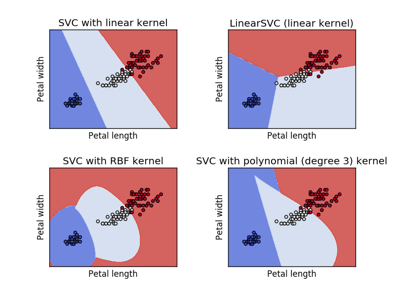
If we run the above code, we will get the below graph. From which we can understand how well different kernel svm classifiers are modeled.
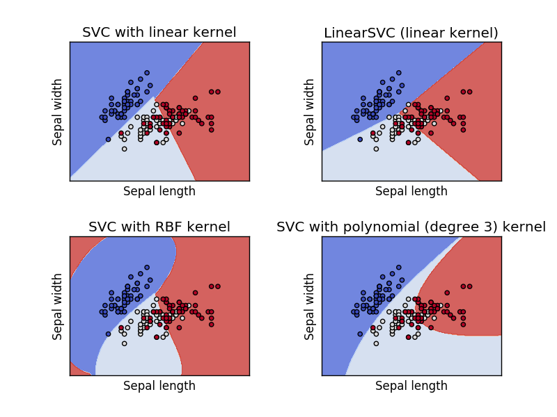
Svm Classifier with Iris Sepal features
From the above graphs, you can clearly understand how different kernel modeled with the same svm classifier. Now let’s model the svm classifier with Petal features using the same kernel we have used for modeling with Sepal features.
Modeling Different Kernel Svm classifier using Iris Petal features
iris = datasets.load_iris()
X = iris.data[:, 2:]  # we only take the last two features.
y = iris.target
C = 1.0  # SVM regularization parameter

# SVC with linear kernel
svc = svm.SVC(kernel='linear', C=C).fit(X, y)
# LinearSVC (linear kernel)
lin_svc = svm.LinearSVC(C=C).fit(X, y)
# SVC with RBF kernel
rbf_svc = svm.SVC(kernel='rbf', gamma=0.7, C=C).fit(X, y)
# SVC with polynomial (degree 3) kernel
poly_svc = svm.SVC(kernel='poly', degree=3, C=C).fit(X, y)
The above code is much similar to the previously modeled svm classifiers code. The only difference is loading the Petal features into X variable. The remaining code is just the copy past from the previously modeled svm classifier code.
Now let’s visualize the each kernel svm classifier to understand how well the classifier fit the Petal features.
Visualizing the modeled svm classifiers with Iris Petal features
h = .02  # step size in the mesh
# create a mesh to plot in
x_min, x_max = X[:, 0].min() - 1, X[:, 0].max() + 1
y_min, y_max = X[:, 1].min() - 1, X[:, 1].max() + 1
xx, yy = np.meshgrid(np.arange(x_min, x_max, h),
	            np.arange(y_min, y_max, h))
# title for the plots
titles = ['SVC with linear kernel',
	  'LinearSVC (linear kernel)',
	  'SVC with RBF kernel',
	  'SVC with polynomial (degree 3) kernel']


for i, clf in enumerate((svc, lin_svc, rbf_svc, poly_svc)):
    # Plot the decision boundary. For that, we will assign a color to each
    # point in the mesh [x_min, x_max]x[y_min, y_max].
    plt.subplot(2, 2, i + 1)
    plt.subplots_adjust(wspace=0.4, hspace=0.4)

    Z = clf.predict(np.c_[xx.ravel(), yy.ravel()])

    # Put the result into a color plot
    Z = Z.reshape(xx.shape)
    plt.contourf(xx, yy, Z, cmap=plt.cm.coolwarm, alpha=0.8)

    # Plot also the training points
    plt.scatter(X[:, 0], X[:, 1], c=y, cmap=plt.cm.coolwarm)
    plt.xlabel('Petal length')
    plt.ylabel('Petal width')
    plt.xlim(xx.min(), xx.max())
    plt.ylim(yy.min(), yy.max())
    plt.xticks(())
    plt.yticks(())
    plt.title(titles[i])

plt.show()
If we run the above code, we will get the below graph. From which we can understand how well different kernel svm classifiers are modeled.
Svm Classifier with Iris Petal features
This is how the modeled svm classifier looks like when we only use the petal width and length to model. With this, we came to an end. Before put an end to the post lets quickly look how to use the modeled svm classifier to predict iris flow categories.
Predicting iris flower category
To Identify the iris flow type using the modeled svm classifier, we need to call the predict function over the fitted model. For example, if you want to predict the iris flower category using the lin_svc model. We need to call lin_svc.predict(with the features). In our case, these features will include the sepal length and width or petal length and width. If you are not clear with the using the predict function correctly you check knn classifier with scikit-learn.
Conclusion
In this article, we learned how to model the support vector machine classifier using different, kernel with Python scikit-learn package. In the process, we have learned how to visualize the data points and how to visualize the modeled svm classifier for understanding the how well the fitted modeled were fit with the training dataset.
Related Articles
- Introduction to support vector machine classifier
- support vector machine classifier implementation in R programming language
Follow us:
FACEBOOK| QUORA |TWITTER| GOOGLE+ | LINKEDIN| REDDIT | FLIPBOARD | MEDIUM | GITHUB
I hope you like this post. If you have any questions, then feel free to comment below. If you want me to write on one particular topic, then do tell it to me in the comments below.
Related Courses:
Do check out unlimited data science courses
| Title of the course | Course Link | Course Link |
Machine Learning: Classification |
Machine Learning: Classification |
|
Data Mining with Python: Classification and Regression |
Data Mining with Python: Classification and Regression |
|
Machine learning with Scikit-learn |
Machine learning with Scikit-learn |
|


Hi I’m not able to predict . How do i pass the parameter to a lin_svr.predict(). please do needful.
Hi Vilas,
You need to pass the same features data for modeling into the predict method. The below article will help you to understand the same.
Link: https://dataaspirant.com/random-forest-classifier-python-scikit-learn/
Thanks! & Happy Learning
i tried to use this code but i got an error message “syntax error: invalid syntax”
def visuvalize_sepal_data():
iris = datasets.load_iris()
X = iris.data[:, :2] # we only take the first two features.
y = iris.target
plt.scatter(X[:, 0], X[:, 1], c=y, cmap=plt.cm.coolwarm)
plt.xlabel(‘Sepal length’)
plt.ylabel(‘Sepal width’)
plt.title(‘Sepal Width & Length’)
plt.show()
visuvalize_sepal_data()
Hi Abdul,
When you copied the code from the article and pasted in your system, the code indentation has changed and the comment in the code uncommented. Which leads to the syntax error. Please use the below code.
def visuvalize_sepal_data():

	iris = datasets.load_iris()

	X = iris.data[:, :2]  # we only take the first two features.

	y = iris.target

	plt.scatter(X[:, 0], X[:, 1], c=y, cmap=plt.cm.coolwarm)

	plt.xlabel('Sepal length')

	plt.ylabel('Sepal width')

	plt.title('Sepal Width & Length')

	plt.show()
visuvalize_sepal_data()
When you copied the above code, please check the indentation. Let me know if you still face the same issue.
Select ALL the code and then go to format and untabify region. Input 8 for indentation.
Hope it will work.