LSTM: Introduction to Long Short Term Memory

Long Short-Term Memory (LSTM) is a type of recurrent neural network (RNN) that excels in handling sequential data.
Its ability to retain long-term memory while selectively forgetting irrelevant information makes it a powerful tool for applications like speech recognition, language translation, and sentiment analysis.
Using a complex network of gates and memory cells, LSTMs have proven incredibly effective in capturing patterns in time-series data, leading to breakthroughs in fields like finance, healthcare, and more.
Long Short-Term Memory (LSTM)
LSTM was initially introduced by Hochreiter & Schmidhuber in the year 1997, later, LSTM was refined my many researchers.
This article covers all the LSTM learning aspects you need to learn. Please grab a cup of coffee and read the entire article.
Before we go further, let’s see the table of contents of this article.
Introduction to Neural Networks
Neural networks are algorithms that are inspired by human brain behaviour. This means neural network algorithms learn patterns from massive historical or past data to remember those patterns and apply gained knowledge to new data to predict the results.



We have many neural network algorithms, such as
Out of all the networks mentioned above, Artificial Neural Network or ANN is the basic architecture of all other neural networks.
Because whatever concepts are present in the ANN are present in the remaining neural networks with additional features or functions based on their tasks.
For example, CNN is used for image classification, object detection, and RNN is used for text classification (sentiment analysis, intent classification), speech recognition, etc.
Basic neural networks consist of 3 different layers, and all these layers are connected to each other. Every layer has a few numbers of neurons inside it.
Neurons are nothing but the core processing units of the whole network architecture.


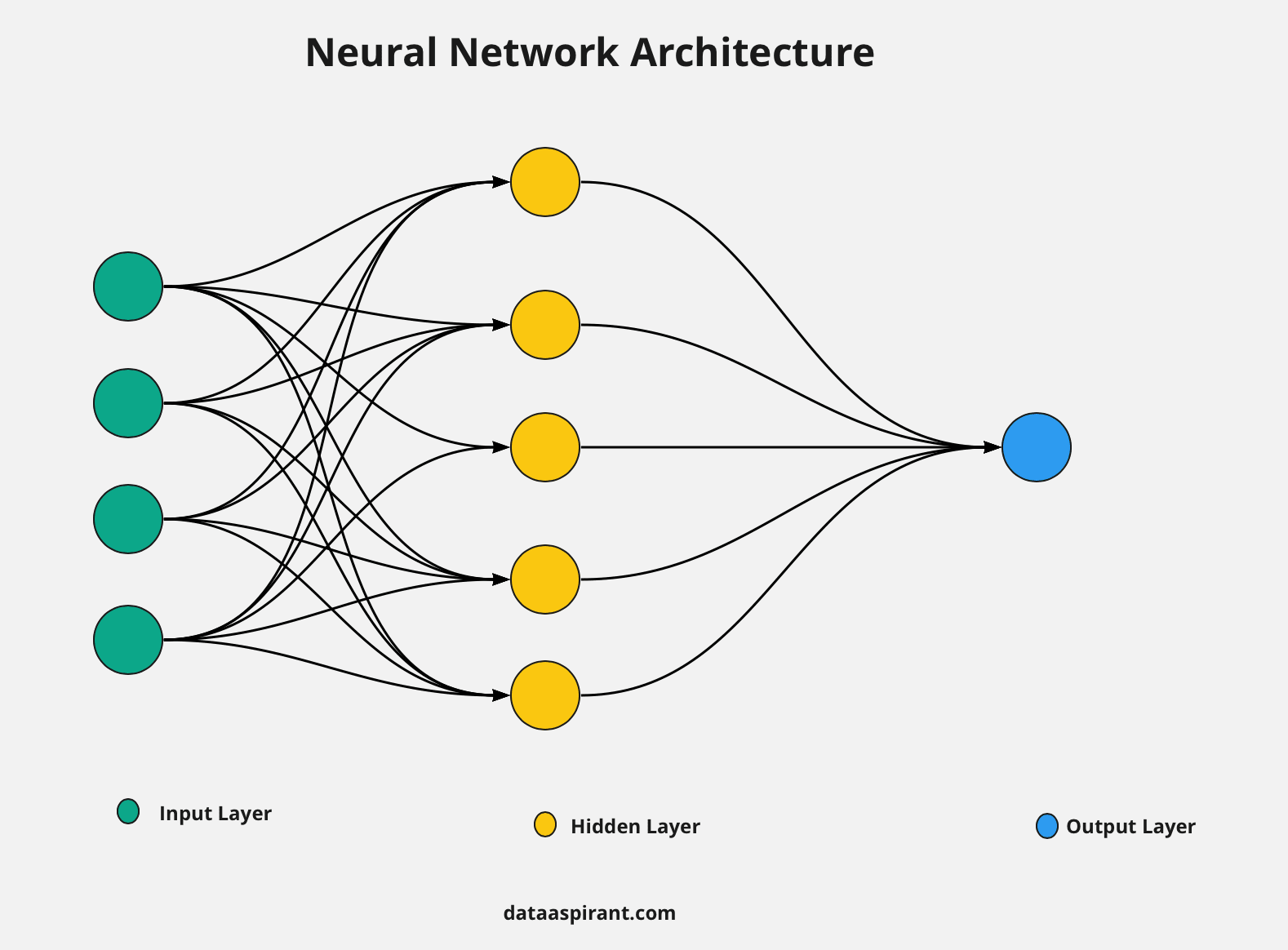

What are the three layers 

- Input Layer
- Hidden Layers
- Output Layer
Input Layer
The input layer takes input as whatever data we have. The number of neurons of an input layer should equal to the number of features present in the data.
The output of an input layer is the same as its input. Neural networks have only one input layer.
Hidden layers
Neural networks may have one or more hidden layers based on the depth of the problem statements or our requirements. The input of hidden layers is the output of previous layers.
This means the first hidden layer takes input as the input layer's output, the second hidden layer takes input as the output of the first hidden layer, and so on.
Output layer
The output layer takes input as the output of the final hidden layer, and this layer has several neurons which are equal to the target labels.
Neural network architecture has additional variable values and functions between each layer to process our data according to the task. Such as
- Weights,
- Bias,
- Activation functions,
- Learning rate.
Neural networks are mainly used for machine learning classification and regression problems.
In traditional neural networks, all inputs and outputs are independent of each other.
Let me explain with an example If we are building a model for credit card fraud detection. Each user data is an input for the model. Each user's data is not dependent on other users' data.
This means the neural network doesn't store knowledge of the previous input or user data while processing the current user data.
We know Neural networks don't have any knowledge of the previous inputs, so how can we predict the next word when we build a model for predicting the next word based on previous words?
Does this mean how we can process sequence data?
To avoid this problem, we have another set of neural network architectures which help build sequence models for processing the sequential data, such as
- Recurrent neural networks
- Long short-term memory network
- Bidirectional Long Short term memory networks
- GRU
- Encoder decoders
- Attention models
- Transformers
- Bert
Before we learn about LSTM, we need to know how RNN works. So let’s spend some time understanding these concepts.
Introduction to Recurrent Neural Network (RNN)
Recurrent Neural Network (RNN ) is a neural network type that takes input as the previous and current step inputs. This is a generalisation feedforward neural network that has an internal memory unit.


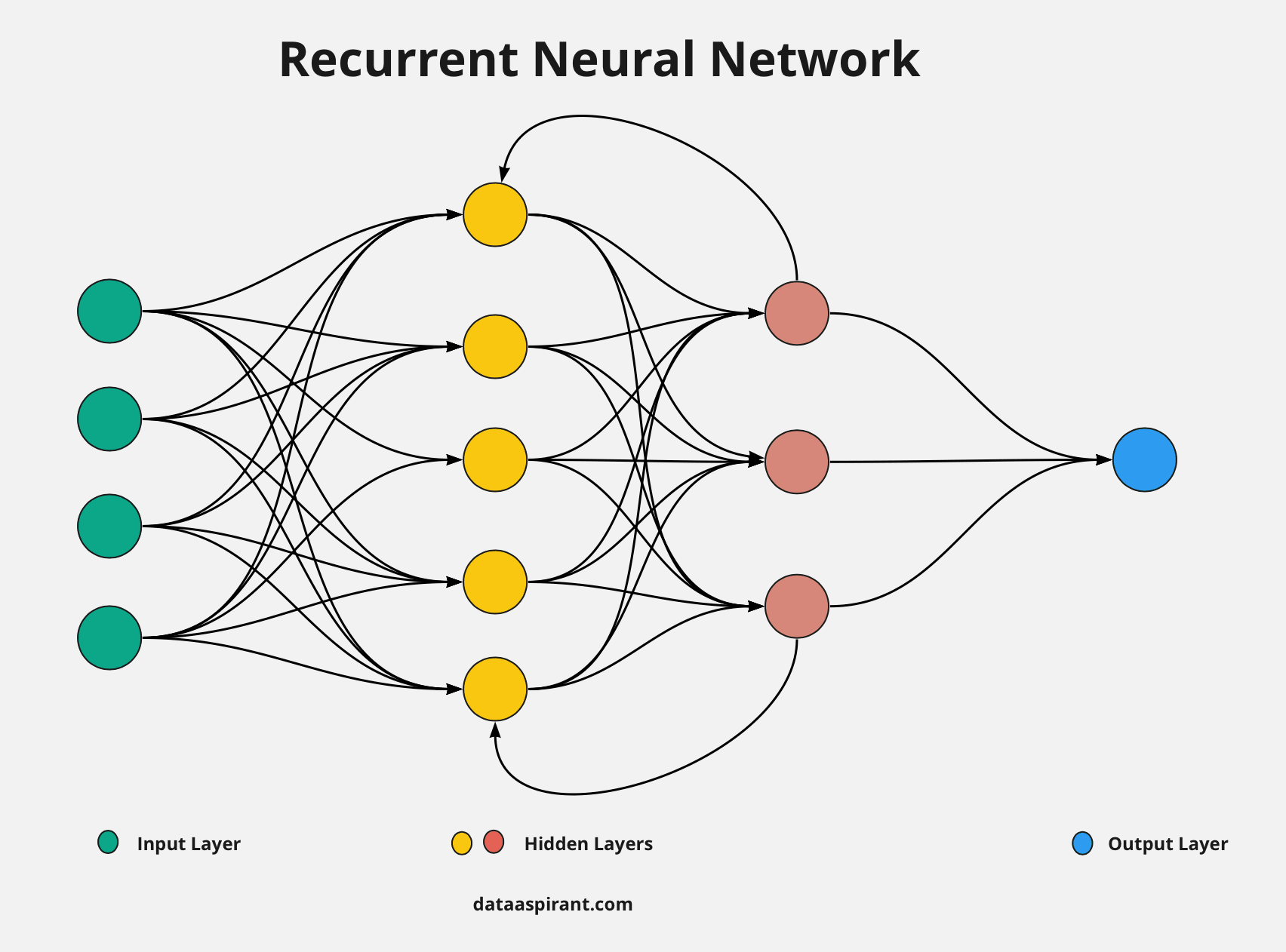

Recurrent means the re-occurrence of the same function, which means RNN performs the same operational function in each module/input.
And also, RNN shares weights and bias values within every time stamp, called parameter sharing. It will reduce the number of parameters & complexity of parameters. Unlike ANN, all the inputs of RNN are dependent on each other.
When predicting the next word or character, the knowledge of the previous data sequence is important. RNN can handle sequences of data.
Examples of sequence data are
- Sentences or text,
- Audio,
- Video.
How Can RNN Handle Sequence Data
RNN has a sequence memory mechanism that makes remembering sequence data easier to recognise sequence patterns.
Using this internal memory unit RNN will store information about previous words, and then it can predict the current word based on previous word information.
But RNN fails at predicting the current output if the distance between the current output and relevant information in the text is large. Because RNN suffers from short-term memory, RNN can't carry information from earlier time stamps to later ones if the sequence's length is long enough.
For example, if you are trying to predict any result from a long paragraph, RNN may lose important information from the beginning of the paragraph.
RNNs work very well when problem statement data or inputs have short text, but it has few limitations in processing long sequences data.
Here LSTM networks come into play to overcome these limitations and effectively process the long sequences of text or data.
In the next section, we will focus on RNN limitations and where exactly RNN fails.
Limitations of RNN
Sometimes language models predict the next word based on previous words, only enough to look at the most recent words/information to predict the next word.
For example :
- The clouds are in the _______.
Suppose you try to predict the last word using the language model in the above example sentence.
In that case, RNN can predict the output because the sentence is small, and the distance between the result place(____) and relevant information (clouds) is also small.
But in some cases, RNN fails when this gap/distance is significant.
For example :
- I have been staying in Spain for the last 20 years. I can speak fluently ______.
The resulting word will depend on the previous words in the sentence. Here our model needs Spain's context when we need to predict the last word; the most suitable word as a result/output is Spanish.
Key RNN limitations
- Slow computation
- Difficult to access the relevant information from a long time ago
- RNN couldn’t consider future information to predict the current output.
- Another limitation of the RNN is that RNN networks suffer from vanishing gradient problems when applying backpropagation on RNN architectures.
Let's see gradient problems and the solution to avoid these limitations in the next few minutes.
Gradient Problems




You are already familiar with this term when you have some knowledge of neural networks. Otherwise, gradients are values used in the model's training phase to update weights to reduce the model error rate.
RNN suffer from 2 kinds of gradient problems such as
- Vanishing Gradient Problem
- Exploding Gradient Problem
Because of these problems, RNN cannot capture the relevant information from long-term dependencies because of multiplicative gradient values that can gradually increase/decrease based on the number of hidden layers.
Vanishing Gradient Problem
We already discussed gradients carrying information in the neural network (RNN). If the gradient value becomes too small, the updated weight values are also small or insignificant.
It takes too much time to train a model, and it is even challenging to learn long data sequences.
Exploding Gradient Problem
The exploding gradient problem is opposite to the vanishing gradient problem; if the gradient value becomes too large, the updated weight values are too big.
Because of this, we may need to include some range of values that may improve model performance. This gradient problem is called the exploding gradient problem.
Poor model performance, less accuracy value, and long training time are the significant issues we can get due to these gradient problems.
Super Power of LSTM Over RNN
LSTM(Long-Short-Term-Memory) is one of the family or a special kind of recurrent neural network (RNN). LSTM can be a default behaviour to learn long-term dependencies by remembering essential and relevant information for a long time.


Let's discuss the extra features of LSTM over RNNs.
If we have a list of tasks or appointments, we must prioritise the tasks; otherwise, we may need help to do essential tasks. And then, we have to add extra space to list equal priority tasks if any task is cancelled.
In RNNs, to add new information to the RNN networks, RNNs apply a function to the existing information. This process completely modifies the existing information.
After this process, we can't identify which is important and which is not important information.
When we come to LSTM, LSTM applies a few modifications like addition & multiplication on the existing information to get new information.
In the LSTM, complete information that is existing and new information flows through a new mechanism called cell states.
Using this mechanism, LSTM can select important information and forget unimportant information. The cell state works as a conveyor belt to transform information from the previous module to the next module.
Every cell state depends on three different dependencies. There are
- Previous cell state (the information which one is stored at the end of the previous time step)
- Previous hidden state ( same as the output of the previous cell)
- Input at the current time step (the new information/input at the present time step).
We will discuss all these things in detail in the coming sections. Before going deeper into LSTM architecture, you have to know what kind of problems are solved by the LSTM.
Following that, you can get more interested to know the architecture and functionalities of the LSTM.
Applications of LSTM




- Image Captioning: Image captioning is the task of generating captions for input images.
- Machine Translation: Machine translation is the process of converting source language to destination language means one language to another language automatically.
- Music Generation: Music is the mixing of different frequencies of various tones. Music generation is a challenging task in the AI world; the music generation model is composing a tiny bit of music with minimum interaction of humans.
- Automating Handwriting Generation: Generating human-like handwriting text from an input written text written by the human.
There are many exciting use cases and applications of LSTM in every industry and also in our daily life. The above applications are more popular and basic applications. Let's understand the standard architecture of the LSTM in the following section.
LSTM Architecture
Long Short Term Memory networks are generally called LSTM. LSTMs are specially built to avoid long-term dependencies. It has the capability of remembering the relevant information for a long period of time as a default behaviour.
Recurrent Neural Networks (RNNs) architecture has a chain of repeating neural networks. This repeating module has a simple and single function: the tanh activation function.


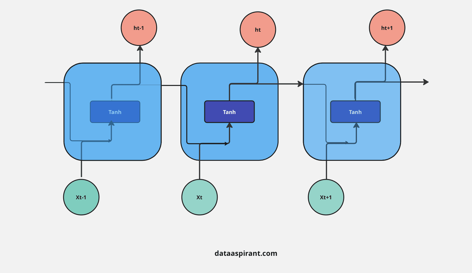

LSTM architecture is also the same as the RNNs, a chain of repeating modules/neural networks. But instead of having only one tanh layer, LSTM repeating models have four different functions.
These four functional operations are especially connected. There are
- Sigmoid Activation Function
- Tanh Activation Function
- Pointwise Multiplication
- Pointwise Addition


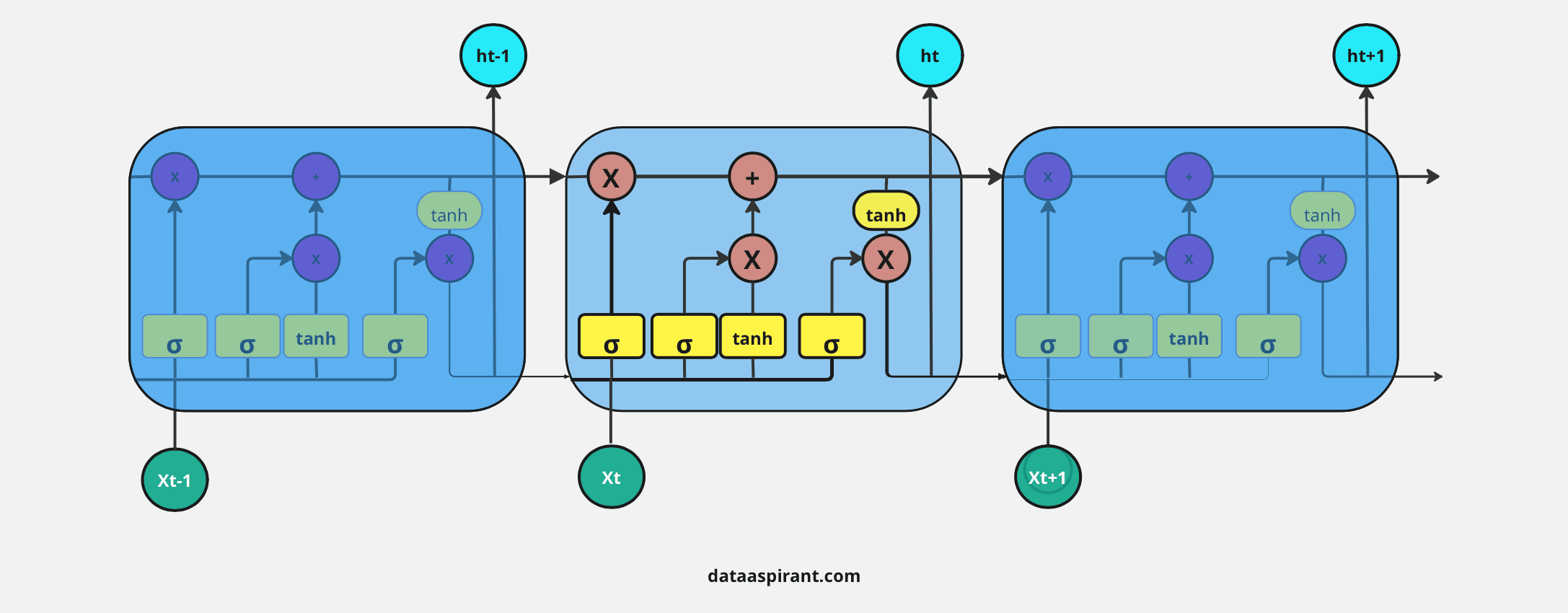

In the whole network, information is transferred in a vector form. Let's discuss the different signs mentioned in the above diagram
- Square Box: a single neural network
- Circle: pointwise operation means the operation is performed element by element
- Arrow Mark: vector information is transformed from one layer to another layer
- Joining two lines into one line: concatenate two vectors
- Splitting one line into two lines: transferring the same information into two different operations or layers.
Don’t worry about all these terms and functions and how the information flows through complete LSTM architecture. We will walk through all these details in the coming sections.
First, let's discuss the main functions and operations in the LSTM architecture.
Activation Functions and Linear Operations Used In LSTM



Sigmoid Function


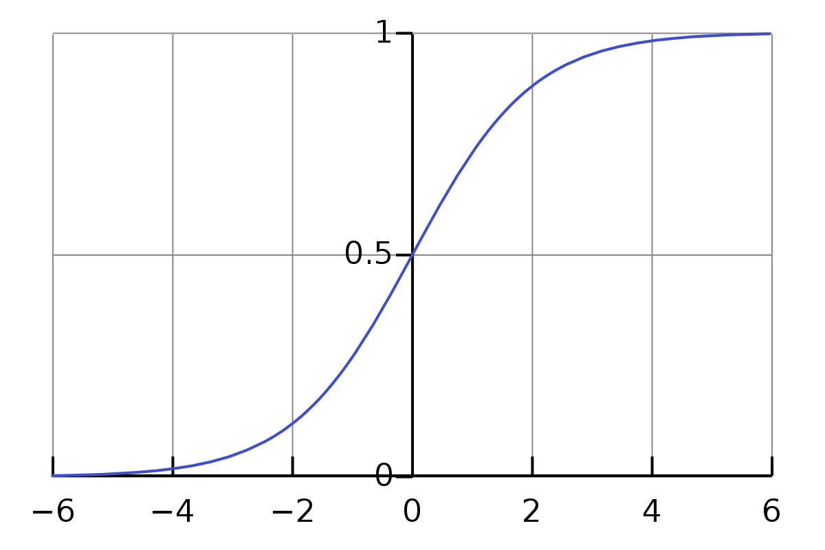

The sigmoid function is also known as the logistic activation function. This function has a smooth and ‘S’ shape curve.
The output results of a sigmoid are always in the range of 0 and 1.
The sigmoid activation function is mainly used for models where we must predict the probabilities as outputs. Since the probability of any input exists only between the range of 0 and 1, the sigmoid or logistic activation function is the right and best choice.
Tanh Activation Function


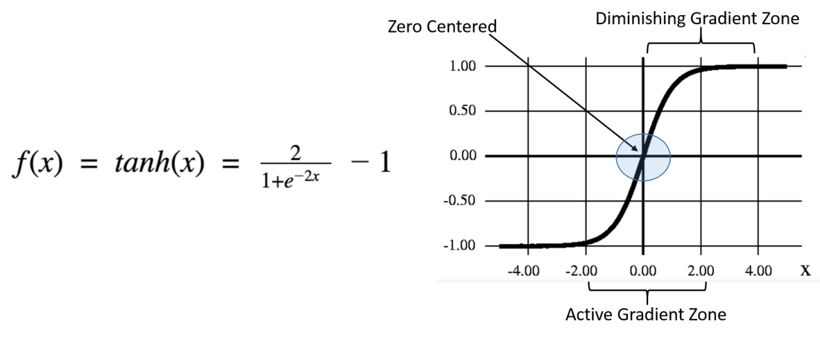

Tanh activation function also looks similar to the sigmoid/logistic function. Actually, it is a scaled sigmoid function. We can write the tanh function formula as a sigmoid function.
The range of tanh function result values are -1 to +1. Using this tanh function, we can find strongly positive, neutral, or negative input.
Pointwise Multiplication
Pointwise multiplication of two vectors is applying multiplication operations on both vectors of individual elements. For example
- A = [1,2,3,4]
- B = [2,3,4,5]
- Pointwise multiplication result : [2,6,12,20]
Pointwise Addition
Pointwise addition of two vectors is the process of adding two vector elements individually. For example
- A = [1,2,3,4]
- B = [2,3,4,5]
- Pointwise addition result : [3,5,7,9]
The Key Concept Behind the LSTM Algorithm
The primary unique behaviour of an LSTM is the cell state; it acts as the conveyor belt with some minor linear interactions.
This means this cell state moves the information with basic operations like addition and multiplication; that's why information smoothly flows along with the cell state without too many changes compared to their original one.
Cell state or a conveyor belt of LSTM is the highlighted horizontal line in the below image.


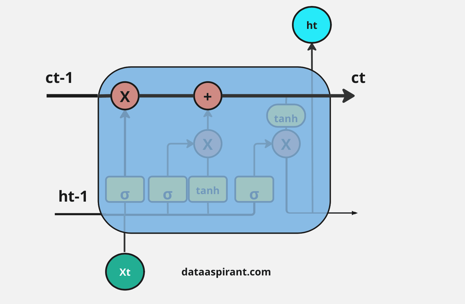

LSTMs have unique structures to identify which information is essential or not important. LSTMs can remove or add information to the cell state based on importance. These special kinds of structures are called gates.
Gates are a unique way to transform information, and LSTMs use these gates to decide which information is to remember, remove, and pass to another layer, etc.
LSTM will remove or add information to the conveyor belt(cell state) based on this information. Every gate comprises a sigmoid neural net layer and a pointwise multiplication operation.
LSTMs have three kinds of gates. There are
- Forget Gate
- Input Gate
- Output Gate
Forget Gate
In the repeating module of the LSTM architecture, the first gate we have is the forget gate. This gate's primary task is to decide which information should be kept or thrown away.
This means deciding which information to send to the cell state to process further. Forget gate takes input as information from the previous hidden state and current input and combines both state's information, and sends it through the sigmoid function.
Results of the sigmoid function between 0 and 1. If a result is closer to 0 means to forget, and if a result is closer to 1 means to keep/remember.
Input Gate
LSTM architecture has an input gate to update the cell state information after the forget gate. Input gates have two kinds of neural net layers one is sigmoid, and another one is tanh. Both network layers take input as previously hidden state information and information from the current input.
Sigmoid network layer results range between 0 and 1, and tanh results range from -1 to 1. The sigmoid layer decides which information is important to keep, and the tanh layer regulates the network.
After applying sigmoid and tanh functions on hidden and current information, then we multiply both outputs. And finally, the sigmoid output will decide which information is important to keep from the tanh output.
Output Gate
The last gate in the LSTM is the output gate. The output gate's primary task is to decide what information should be in the next hidden state. This means the output layer's output is the input to the next hidden state.
The output gate also has two neural net layers, the same as the input gate. But the operations are different. From the input gate, we got updated cell state information.
We have to send hidden state and current input information through the sigmoid layer and updated cell state information through the tanh layer in this output gate. And then multiply both results of the sigmoid and tanh layers.
The final result is sent to the next hidden layer as the input.
Step-by-step Working Procedure of LSTM
The first and foremost step in the LSTM architecture is to decide which information is essential and which is thrown away from the previous cell state. The first gate that does this process in the LSTM is the “Forget gate.”
Forget gate takes input as the previous time step is hidden layer information (ht-1) and present time step input (xt) and sends it through the sigmoid neural net layer.
The result is the vector form, which contains 0 and 1 values. And then, apply a pointwise multiplication operation on the previous cell state (Ct-1) information (vector form) and the output of the sigmoid function (ft).
The final result output of the forget gate 1 represents “completely keep this information,” and 0 represents “don’t keep this information.”


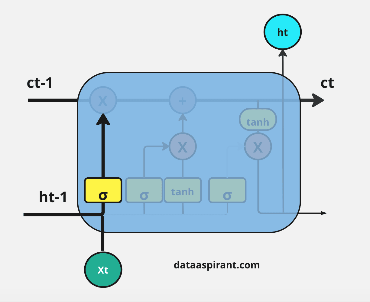

The next step is to decide which information to store in the current cell state (Ct). Another gate will do the task, the second gate in the LSTM architecture is the “Input Gate.”
This whole process of updating the cell state with new important information will be done by using two kinds of activation functions/ neural net layers; their sigmoid neural net and the tanh neural net layer.
First sigmoid net takes the input like the forget gate: previous time step is hidden layer information (ht-1) and current time step (xt).
This process decides which values we’ll update. And then, the tanh neural net also takes the same input as a sigmoid neural net layer. It creates new candidate values in the form of the vector (ct(upper dash)) to regulate the network.


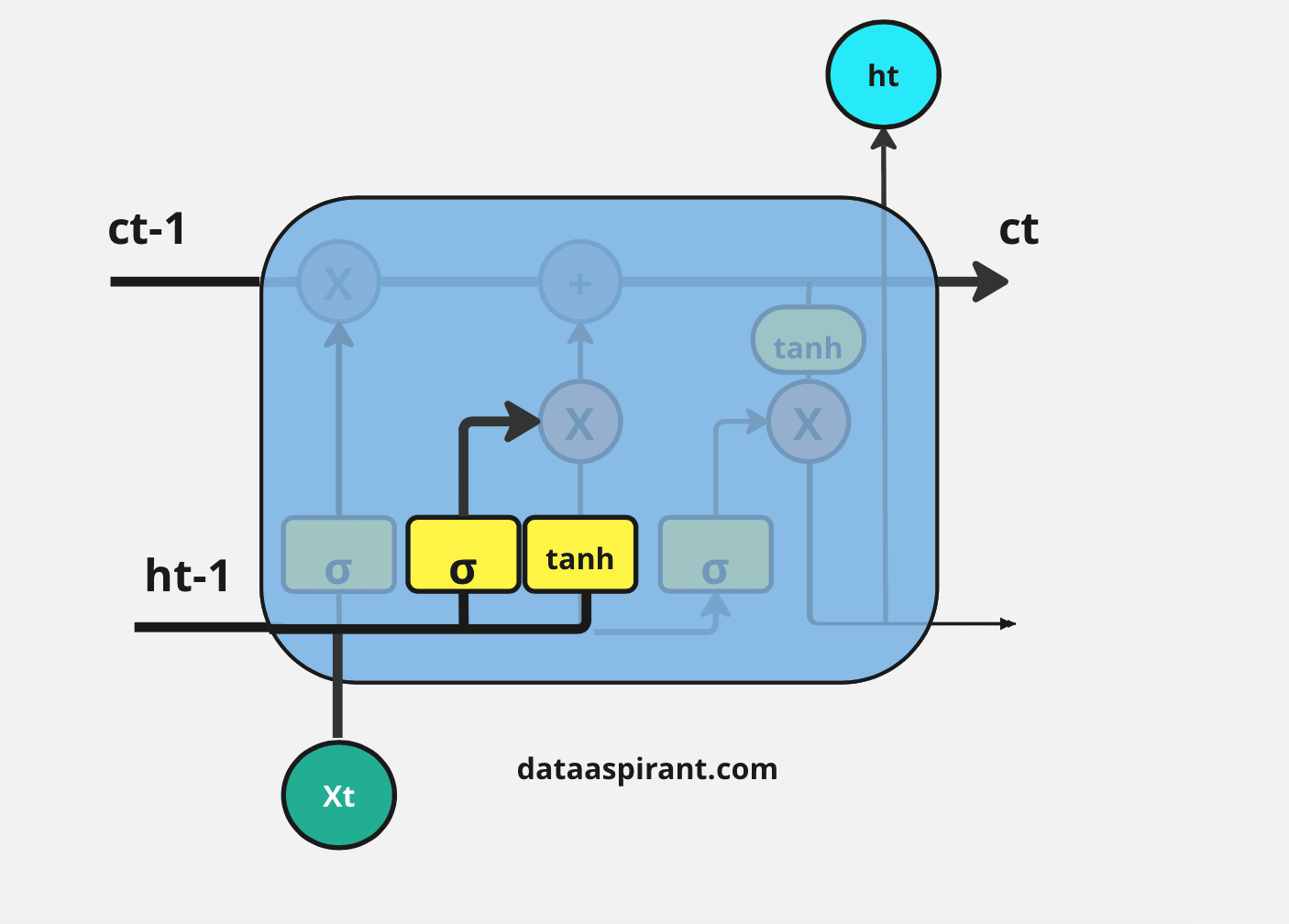

Now we apply pointwise multiplication on the outputs of the sigmoid and tanh layers. After that, we have to perform a pointwise addition operation on the output of the forget gate and the result of the pointwise multiplication in the input gate to update the current cell state information (ct).


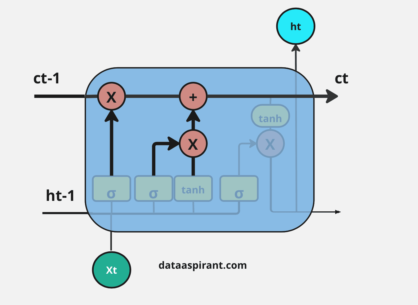

The final step in the LSTM architecture is to decide which information we'll be going to as the output; the final gate that will do this process in the LSTM is the "Output Gate." This output will be based on our cell state but will be the filtered version.
In this gate, we first apply the sigmoid neural net, which takes input like the previous gates' sigmoid layer: previous time step hidden layer information(ht-1) and current time input (xt) to decide what parts of the cell state information going to the output.
And then send updated cell state information through the tanh neural net layer to regulate the network (push the values between -1 and 1) and then apply pointwise multiplication on both results of the sigmoid and tanh neural network layers.


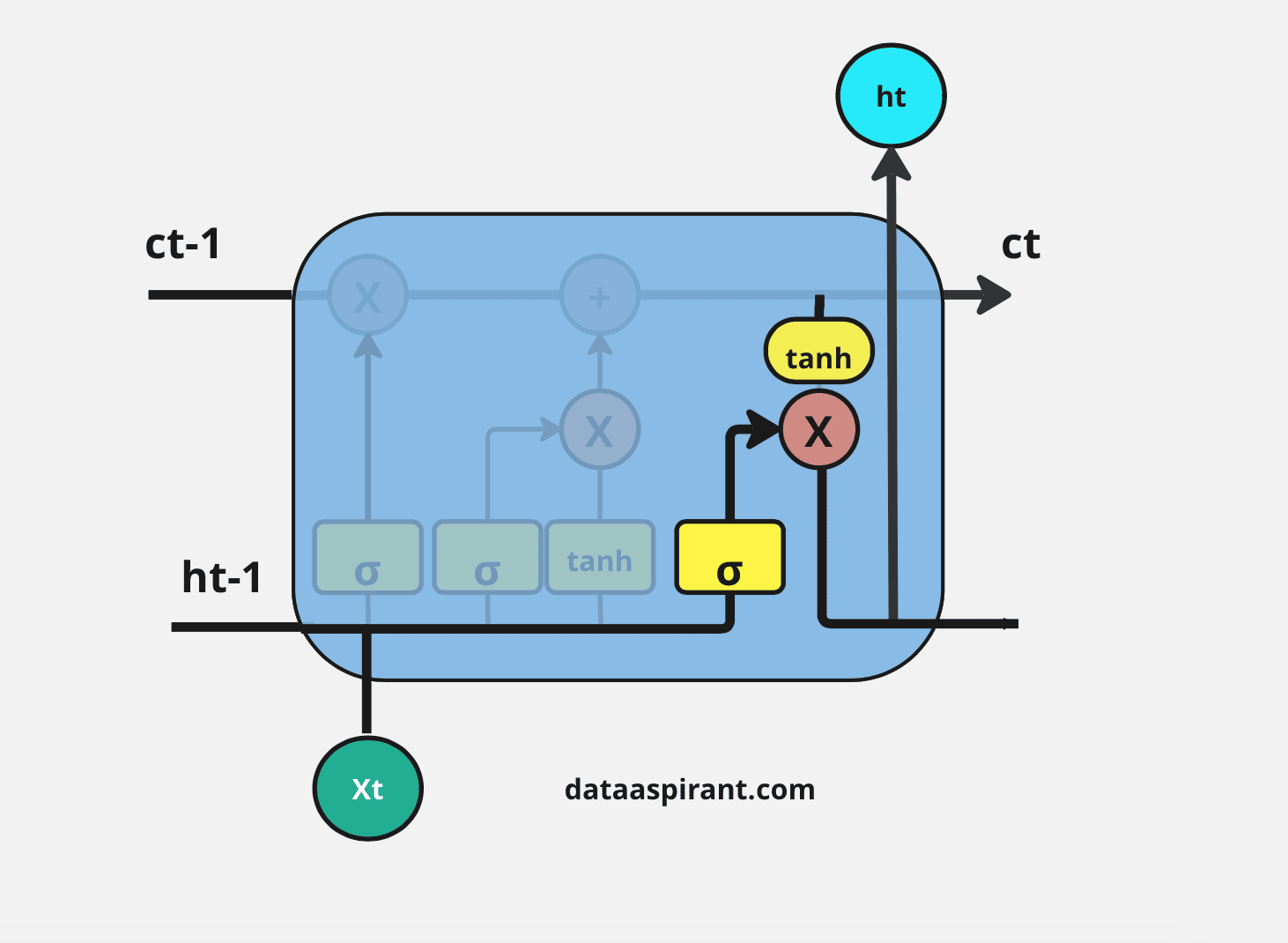

This whole process is repeated in every module of the LSTM architecture.
Different Types of LSTM Architectures
LSTM is the most interesting starting point to solve or address sequence prediction problems. Based on the way LSTM networks are used as layers,
we can divide LSTM architectures into various kinds of LSTMs.


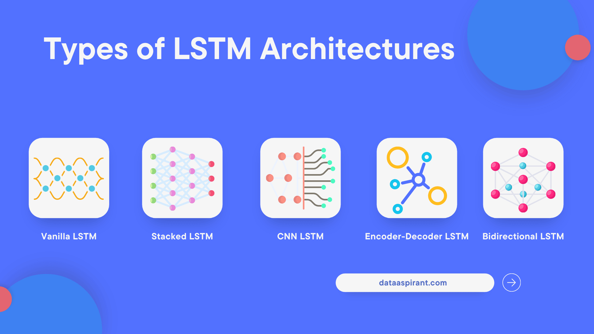

This section will discuss mostly used five different types of LSTM architectures. There are
- Vanilla LSTM architecture
- Stacked LSTM architecture
- CNN LSTM architecture
- Encoder-Decoder LSTM architecture
- Bidirectional LSTM architecture
Vanilla LSTM
Vanilla LSTM architecture is the basic LSTM architecture; it has only one single hidden layer and one output layer to predict the results.
Stacked LSTM
Stacked LSTM architecture is the LSTM network model that compresses a list or multiple LSTM layers. Stacked LSTM is also known as the Deep LSTM network model.
In this architecture, every LSTM layer predicts the sequence of outputs to send to the next LSTM layer instead of predicting a single output value. Then the final LSTM layer predicts the single output.
CNN LSTM
CNN LSTM architecture is a combination of CNN and LSTM architectures. This architecture uses the CNN network layer to extract the essential features from the input and then send them to the LSTM layer to support sequence prediction.
An example application for this architecture is generating textual descriptions for the input image or sequences of images like video.
Encoder-Decoder LSTM
Encoder-decoder LSTM architecture is a special kind of LSTM architecture. It is mainly designed to solve sequence-to-sequence problems such as machine translation, speech recognition, etc. Another name for encoder-decoder LSTM is seq2seq (sequence to sequence).
Sequence-to-sequence problems are challenging problems in the Natural language processing field because, in these problems, the number of input and output items can vary.
Encoder-decoder LSTM architecture has an encoder to convert the input to an intermediate encoder vector. Then one decoder transforms the intermediate encoder vector into the final result. Both the encoder and decoder are stacked LSTMs.
Bidirectional LSTM
Bidirectional LSTM architecture is the extension of traditional LSTM architecture. This architecture is more suitable for sequence classification problems such as sentiment classification, intent classification, etc.
Bidirectional LSTM architecture uses two LSTMs instead of one LSTM one is for forwarding direction (from left to right) and another LSTM for backward direction (from right to left).
This architecture can provide more context information to the network than the traditional LSTM because it will gather information of a word from both sides, the left and right sides. It will accelerate the performance of the sequence classification problems.
Conclusion
In conclusion, Long Short-Term Memory (LSTM) is a remarkable type of recurrent neural network (RNN) that has revolutionized the field of sequential data analysis.
By introducing memory cells and gating mechanisms, LSTMs can selectively retain important information while discarding irrelevant data, making them extremely effective in capturing patterns and long-term dependencies in time-series data.
As a result, LSTMs have become a popular tool in various domains, including natural language processing, speech recognition, and financial forecasting, among others.
Despite their power, LSTMs are not without limitations, and ongoing research is exploring ways to improve their performance and efficiency.
Frequently Asked Questions (FAQs) On LSTM
1. What is LSTM in Machine Learning?
LSTM stands for Long Short-Term Memory. It’s a type of recurrent neural network (RNN) architecture used in deep learning that is designed to remember long-term dependencies in sequential data.
2. How Does LSTM Differ From Traditional Neural Networks?
Unlike traditional neural networks, LSTMs have a unique structure that allows them to effectively capture long-term dependencies and avoid the vanishing gradient problem common in standard RNNs.
3. What Makes LSTM Suitable for Sequential Data?
LSTMs are designed with special units called gates that regulate the flow of information. These gates help the network to retain important long-term information and forget irrelevant data, making them ideal for tasks involving sequential data like time series analysis or natural language processing.
4. Can You Explain the Structure of an LSTM Unit?
An LSTM unit includes three gates: the input gate (controls the flow of input signals), the forget gate (decides what information should be thrown away), and the output gate (determines what the next hidden state should be).
5. What are the Common Applications of LSTM?
LSTMs are widely used in language modeling, machine translation, speech recognition, time series forecasting, and anomaly detection in sequential data.
6. How Does LSTM Handle the Vanishing Gradient Problem?
LSTMs handle the vanishing gradient problem through their gate structure which allows gradients to flow unchanged. This structure helps in maintaining the gradient over many time steps, thereby preserving long-term dependencies.
7. What is the Difference Between LSTM and GRU?
GRU (Gated Recurrent Unit) is a variation of LSTM. It combines the forget and input gates into a single “update gate” and merges the cell state and hidden state, making it simpler and often faster to train than LSTM.
8. Is LSTM Good for Time Series Forecasting?
Yes, LSTMs are particularly effective for time series forecasting tasks, especially when the series has long-range temporal dependencies.
9. Can LSTM be Used for Classification Tasks?
Absolutely. LSTMs can be used for sequence classification tasks such as sentiment analysis or classification of time series data.
10. What is Bidirectional LSTM?
A Bidirectional LSTM processes data in both forward and backward directions, which can provide additional context and improve model performance on certain tasks like language translation.
11. How Resource-Intensive is LSTM Training?
Training LSTMs can be computationally intensive due to their complex architecture, particularly for large datasets or long sequences.
12. What are Some Best Practices for Training LSTM Models?
Best practices include using a proper regularization technique to prevent overfitting, choosing an appropriate optimizer, and preprocessing data effectively. It's also important to experiment with different architectures and tuning hyperparameters.
13. How Do You Choose Between LSTM and Other Deep Learning Models?
The choice depends on the specific task and the nature of the data. LSTMs are ideal for problems where understanding long-term dependencies is crucial.
14. Can LSTMs Process Multi-Dimensional Data?
While LSTMs are inherently designed for one-dimensional sequential data, they can be adapted to process multi-dimensional sequences with careful preprocessing and model design.
Recommended Courses


Deep Learning Course
Rating: 4.5/5




NLP Course
Rating: 4/5


Machine Learning Course
Rating: 4/5


