Popular Dimensionality Reduction Techniques Every Data Scientist Should Learn

Have you ever encountered the term "Dimensionality Reduction Techniques" and skipped it, thinking it's too complicated?
Fear not! You should only skip YouTube ads; Not our content 🙂
In today's article, I'll demystify "Dimensionality Reduction" for you in the simplest way possible!
Dimensionality reduction techniques are an essential component of modern data analysis, particularly in the era of big data, where datasets often consist of a large number of features or variables.
The primary goal of these techniques is to simplify complex datasets by reducing the number of dimensions while preserving the inherent structure and relationships within the data.
Popular Dimensionality Reduction Techniques
This makes the data more manageable and improves subsequent analysis, modeling, and visualization efficiency and interpretability. This comprehensive guide will delve into the world of Dimensionality reduction techniques, exploring various methods, their underlying principles, and practical applications across a wide range of domains.
By understanding these techniques in-depth, you will be better equipped to handle large and complex datasets, extract meaningful insights, and make well-informed decisions in your data-driven endeavours. So, let's embark on this exciting journey into the realm of Dimensionality reduction!
What Is Dimensionality Reduction
Imagine you have a really big toy box filled with lots and lots of toys. Now, sometimes you want to clean up your room, but it's hard to do with all those toys in the way.
So what do you do?
You try to sort them out and put them away, right?



Well, sometimes we have a lot of information in our data, and it can be just like those toys. Too much to handle and too many to make sense of! That's where dimensionality reduction comes in.
It's like sorting through all those toys and figuring out which ones are the most important to keep and which ones can be put away for later.
Dimensionality reduction helps us simplify all that information to see patterns and relationships more clearly. We can use special tools and techniques to pick out the most important parts of the data and put everything else aside. In technical term, feature selection. It's like we're making a smaller, more manageable toy box to play with!
Why do we need it?
Well, sometimes, we have so much data that it's hard to make sense of it all. But with dimensionality reduction, we can make it easier to understand and work with.
It can also help us see things we might have missed or find new insights we didn't even know existed! So, just like cleaning up your toy box can make your room feel better, dimensionality reduction can help make sense of all that information and make it easier to work with.
The Curse of Dimensionality
The curse of dimensionality is a phenomenon that occurs when working with (analyzing and visualizing) data in high-dimensional spaces, which do not exist in low-dimensional spaces.




As a dataset's number of features or factors (also known as variables) increases, visualization and analysis become increasingly challenging. Moreover, many variables are often correlated, leading to redundancy when all variables in the feature set are considered for the training set.
Additionally, as the number of variables grows, so does the required sample size to represent all possible combinations of feature values in the dataset.
This variable increase results in more complex models, raising the likelihood of overfitting. When an ML models are trained on a large dataset with numerous features, it heavily relies on the training data, leading to overfitted models that underperform on real data.
The primary goal of dimensionality reduction is to prevent overfitting. A training dataset with significantly fewer features ensures a simpler model with fewer assumptions.
Dimensionality reduction offers several other benefits, such as:
- Removing noise and redundant features.
- Enhancing the model's accuracy and performance.
- Enabling the use of algorithms that are unsuitable for higher dimensions.
- Reducing the required storage space (fewer data requires less storage).
- Compressing data decreases computation time and facilitates faster training.
Why do we need to use Dimensionality Reduction Techniques?
Dimensionality reduction techniques simplify the feature space by reducing the number of input variables while retaining most of the relevant information.



This is important because real-world datasets often have many features, which can make the analysis process computationally expensive, slow, and sometimes lead to overfitting.
There are two main reasons why dimensionality reduction techniques are used:
- To improve efficiency:
- One of the primary reasons for using dimensionality reduction techniques is to improve the computational efficiency of the machine learning algorithm.
- By reducing the number of input variables, the algorithm can run much faster, which can be crucial when dealing with large datasets or real-time applications.
- To avoid overfitting:
- Another reason for using dimensionality reduction techniques is to prevent overfitting. Overfitting occurs when a model is too complex and it fits the training data too closely, resulting in poor generalization to new data.
- Reducing the number of input variables makes the model less complex and reduces the risk of overfitting.
There are two main approaches to dimensionality reduction:
- Feature Selection:
- In feature selection, we select a subset of the original features that are most relevant to the prediction task. This approach involves ranking the features based on their importance and then selecting the top-ranked features.
- Feature selection can be achieved using statistical methods, such as correlation analysis, or using machine learning methods, such as decision trees.
- Feature Extraction:
- In feature extraction, we transform the original features into a new set of features that are a linear combination of the original features. The new set of features, also known as latent variables, captures the essential information from the original features.
- Principal Component Analysis (PCA) and Linear Discriminant Analysis (LDA) are two popular feature extraction techniques.
Advantages and Disadvantages of Dimensionality Reduction
Dimensionality reduction techniques have several advantages and disadvantages, which can impact their suitability for specific applications.
Let's see the key advantages and disadvantages of dimensionality reduction.


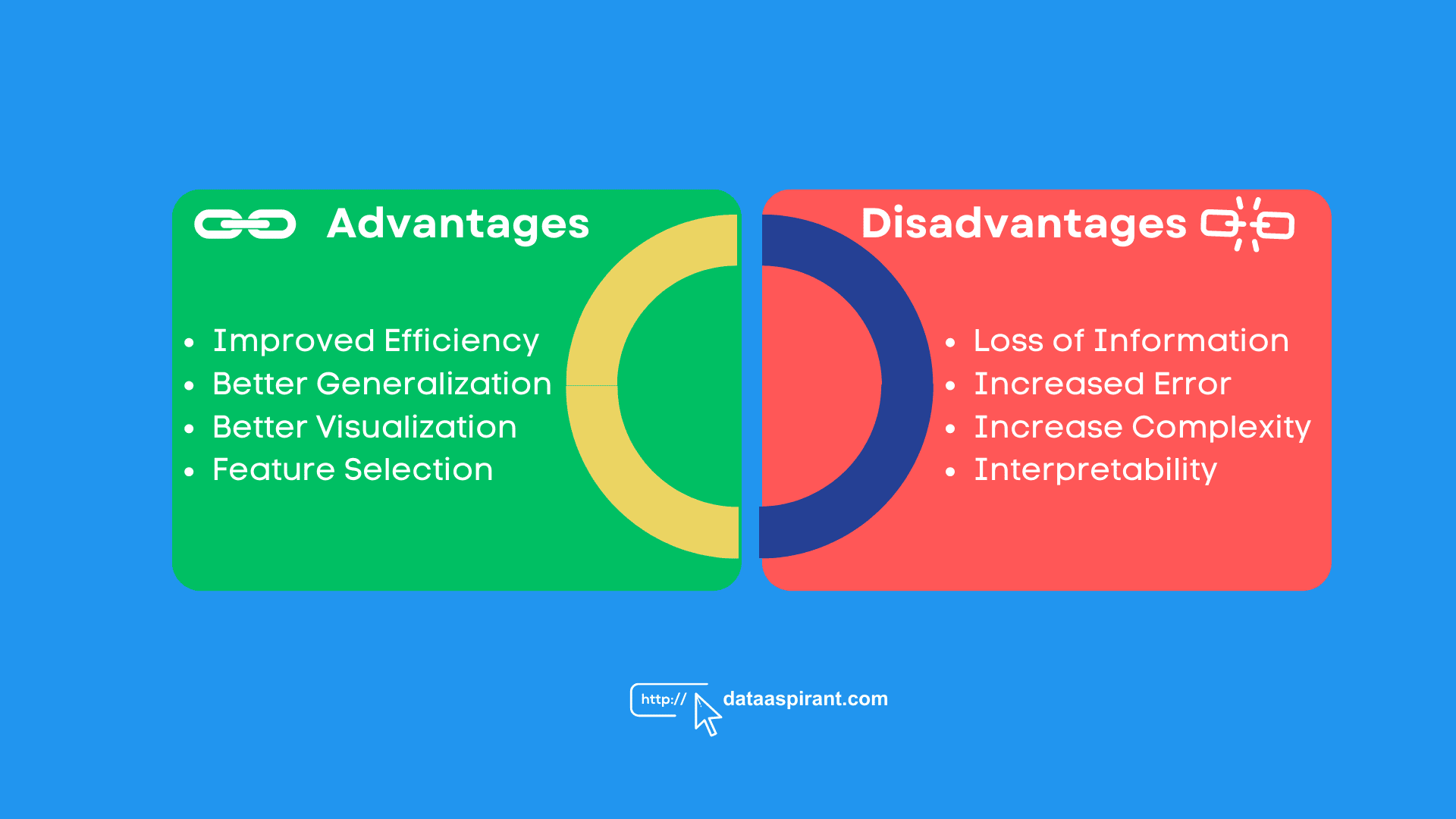

Advantages of Using Dimensionality Reduction Techniques:
- Improved Efficiency: One of the primary advantages of dimensionality reduction is that it can improve the computational efficiency of machine learning algorithms. Reducing the number of input features allows the algorithm to run much faster, which is essential when dealing with large datasets or real-time applications.
- Better Generalization: Dimensionality reduction can also improve the model's generalisation. By reducing the number of features, we can simplify the model and reduce the risk of overfitting. Overfitting occurs when a model is too complex and fits the training data too closely, resulting in poor performance on new data.
- Better Visualization: Dimensionality reduction techniques can also help visualize high-dimensional data. By reducing the number of dimensions, we can plot the data on a two-dimensional or three-dimensional graph, which can help us better understand the structure of the data.
- Feature Selection: Some dimensionality reduction techniques, such as feature selection, can help identify the most relevant features for the prediction task. This can simplify the model and improve its accuracy.
Disadvantages of Using Dimensionality Reduction Techniques:
- Loss of Information: The primary disadvantage of dimensionality reduction is that it can result in a loss of information. By reducing the number of dimensions, we may remove important features that are essential for accurate predictions.
- Increased Error: Sometimes, dimensionality reduction techniques can increase the error rate. This can happen if the reduced feature space is not representative of the original data or if the reduction process is not done correctly.
- Increased Complexity: Some dimensionality reduction techniques, such as non-linear methods, can be computationally intensive and require a lot of resources. This can make them impractical for some applications.
- Interpretability: Dimensionality reduction techniques can also reduce the interpretability of the model. By reducing the number of dimensions, we may lose the ability to understand how the model makes its predictions.
Different Dimensionality Reduction Techniques


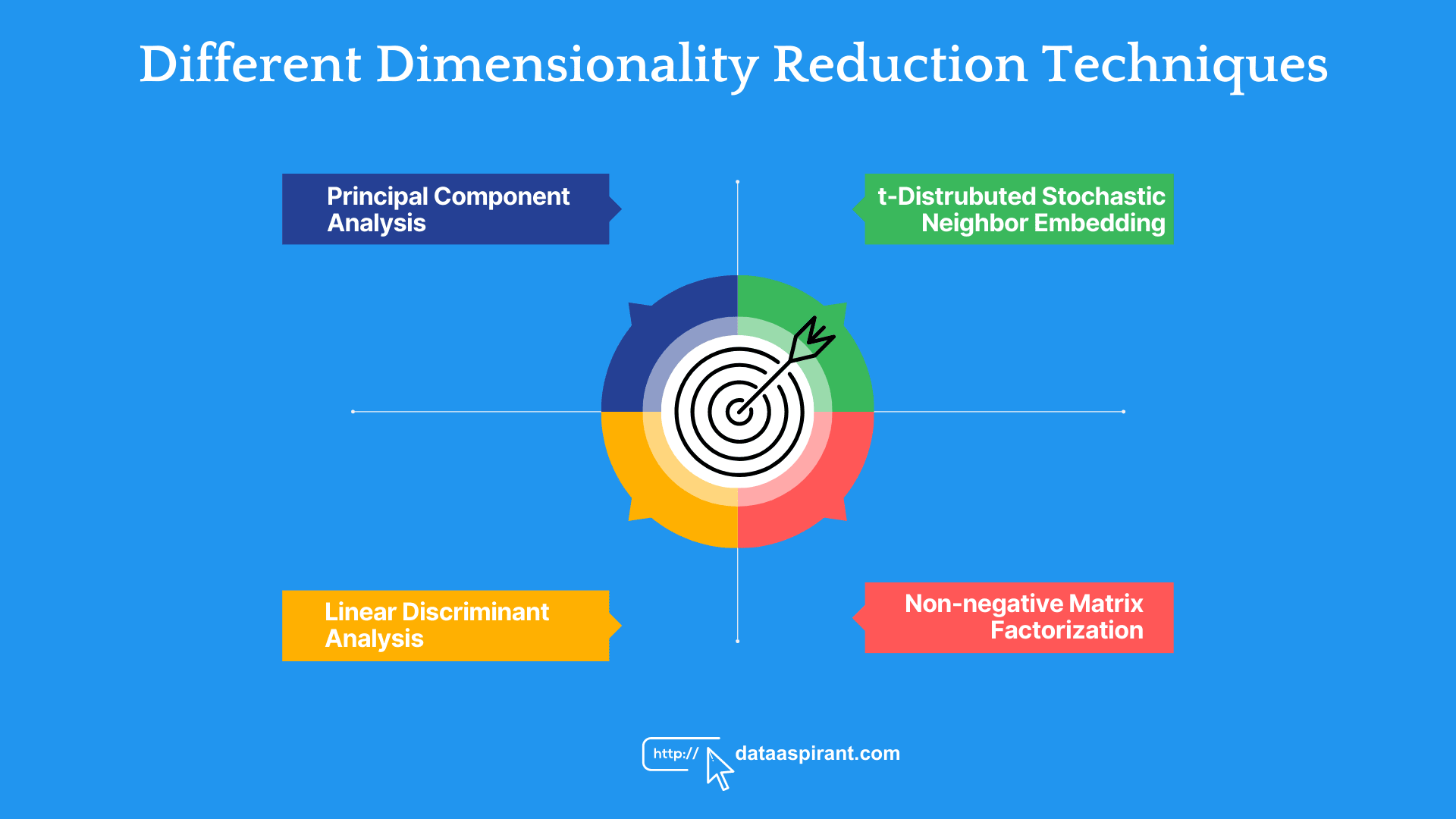

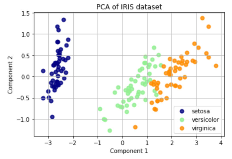
Principal Component Analysis
It's a widely used technique in machine learning and data analysis for reducing the dimensionality of data. In other words, it helps to identify a dataset's most important features or dimensions.
- Here's a simple explanation of how PCA works:
Suppose you have a dataset with many different variables (like height, weight, age, income, etc.). You want to find the most important variables that explain the majority of the variance in the data.
PCA helps to identify these variables by finding new, "artificial" variables that are linear combinations of the original variables. These new variables are called principal components.
The first principal component captures the largest amount of variance in the data, the second principal component captures the second largest amount of variance, and so on.
Once you've identified the principal components, you can use them to reduce the dimensionality of your data. You can keep only the top principal components (i.e. the ones that explain the most variance) and discard the rest.
This can help to simplify your analysis and make it easier to see patterns and relationships in the data.
Now, let's take a look at the mathematical side of PCA:
- Standardization: First, we need to standardize our data so that all the variables have the same scale. This is important because PCA is a variance-based method, and variables with larger variances will have more influence on the principal components.
- Covariance Matrix: Next, we calculate the covariance matrix of the standardized data. The covariance matrix shows how much the variables in the dataset vary together.
- Eigen decomposition: We then perform an eigende composition of the covariance matrix. This gives us the eigenvectors and eigenvalues of the matrix. The eigenvectors are the principal components, and the corresponding eigenvalues represent the amount of variance that each principal component explains.
- Dimensionality Reduction: Finally, we can use the eigenvectors to transform the original data into a new, lower-dimensional space. We can keep only the top principal components (i.e. the ones with the highest eigenvalues) and discard the rest to reduce the dimensionality of the data.



t-Distrubuted Stochastic Neighbor Embedding
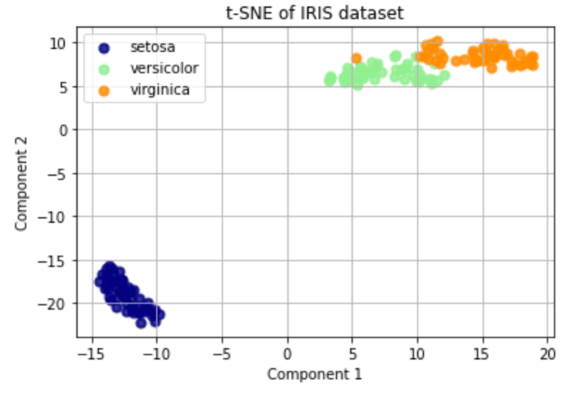
t-SNE is a machine learning technique that is often used for data visualization. It allows you to take high-dimensional data and visualize it in a lower-dimensional space (usually 2D or 3D) so that you can see the relationships between different data points.
Here's a simple explanation of how t-SNE works:
Imagine you have a dataset with many different variables (like height, weight, age, income, etc.). You want to visualize this dataset in 2D or 3D so that you can see the relationships between different data points.
t-SNE works by first creating a probability distribution that represents the relationships between the data points in the high-dimensional space. It then creates a similar probability distribution in the lower-dimensional space.
It tries to minimize the difference between these two probability distributions by adjusting the position of the data points in the lower-dimensional space.
In other words, t-SNE tries to preserve the pairwise similarities between data points in the high-dimensional space as closely as possible in the lower-dimensional space. This allows you to see the structure and relationships in the data, even when many dimensions would make it difficult to visualize directly.
Now, let's take a look at the mathematical side of t-SNE:
Probability Distribution: First, t-SNE creates a probability distribution that represents the pairwise similarities between data points in the high-dimensional space. This is done using a Gaussian distribution that assigns higher probabilities to data points that are closer together.
Low-Dimensional Probability Distribution: t-SNE then creates a similar probability distribution in the lower-dimensional space. This is done using a t-distribution with a single degree of freedom. This distribution has heavier tails than the Gaussian distribution, which helps to spread out the data points in the lower-dimensional space.
Cost Function: t-SNE then minimizes a cost function that measures the difference between these two probability distributions. The cost function measures the Kullback-Leibler divergence between the two distributions.
Gradient Descent: Finally, t-SNE uses gradient descent to adjust the position of the data points in the lower-dimensional space in order to minimize the cost function.



Linear Discriminant Analysis (LDA)
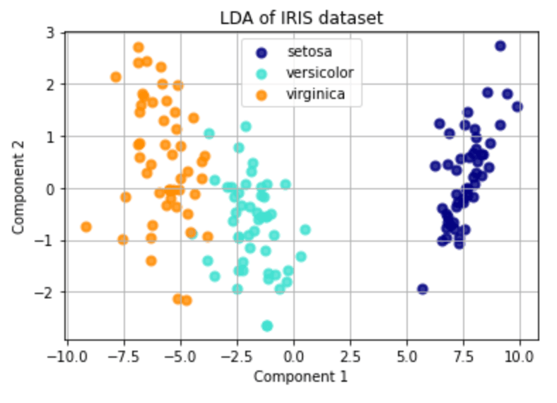
LDA is a machine learning technique that is often used for classification tasks. It works by identifying the linear combination of features (also known as predictors or independent variables) that best separates different classes of data points.
Here's a simple explanation of how LDA works:
Imagine you have a dataset with many different features (like height, weight, age, income, etc.) and you want to classify each data point into one of two or more classes (like "healthy" vs. "sick", or "spam" vs. "not spam").
LDA works by first identifying the linear combination of features that maximizes the separation between the different classes. This is done by calculating the mean and variance of each feature for each class and using these statistics to estimate the likelihood of each class for each data point.
Once this linear combination of features has been identified, it can be used to classify new data points based on which side of the decision boundary they fall on.
Now, let's take a look at the mathematical side of LDA:
Class Means: First, LDA calculates the mean of each feature for each class. This gives us a set of vectors representing each feature's average values for each class.
Within-Class Scatter: LDA then calculates the within-class scatter matrix, which measures the variation of each feature within each class. This is done by calculating the difference between each data point and its class mean and then squaring and summing these differences for each feature.
Between-Class Scatter: LDA also calculates the between-class scatter matrix, which measures the variation of each feature between different classes. This is done by calculating the difference between the mean of each class and the overall mean of the data and then squaring and summing these differences for each feature.
Eigenvalue Decomposition: LDA then performs an eigenvalue decomposition of the matrix that is the product of the inverse of the within-class scatter matrix and the between-class scatter matrix. This gives us a set of eigenvectors and eigenvalues.
Dimensionality Reduction: Finally, LDA selects the top eigenvectors (i.e. the ones with the highest eigenvalues) and uses them to transform the original data into a new, lower-dimensional space. This new space can be used to classify new data points based on their position relative to the decision boundary.



Non-negative Matrix Factorization (NMF)
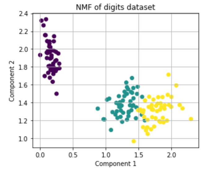
NMF is a machine learning technique that is used for dimensionality reduction and feature extraction. It works by decomposing a large matrix into two smaller matrices that have the property of non-negativity.
This can be useful in various machine learning applications, including image processing, text mining, and speech recognition.
Here's a simple explanation of how NMF works:
Imagine you have a data matrix with many rows (samples) and columns (features). NMF aims to factorize this matrix into two smaller matrices:
- One that contains a small number of basis vectors (also known as components or factors),
- The another that contains a set of coefficients that represent how each sample can be represented as a combination of these basis vectors.
The key feature of NMF is that it enforces the constraint that all elements in the matrices must be non-negative. This allows the basis vectors and coefficients to represent only additive combinations of the original data.
Which can be more interpretable than other linear factorization methods that allow for negative values.
Now, let's take a look at the mathematical side of NMF:
- Data Matrix: First, we start with a matrix X that has dimensions (m x n), where m is the number of samples and n is the number of features.
- Basis Vectors: Next, we assume that k basis vectors (W) can be used to represent the original data. These basis vectors have dimensions (m x k), where k is the number of components.
- Coefficients: We then assume that each sample in X can be represented as a combination of the basis vectors with a set of coefficients (H), which has dimensions (k x n).
- Optimization: The goal of NMF is to find the values of W and H that minimize the error between the original data X and the product of W and H (i.e. X ≈ WH).
- Non-negativity: To enforce non-negativity, NMF uses an iterative algorithm that alternates between updating the values of W and H while constraining all elements to be non-negative.
- Objective Function: The objective function that NMF seeks to minimize is typically based on the Frobenius norm, which measures the squared difference between X and WH.



Conclusion
In conclusion, dimensionality reduction is an essential technique used to simplify the feature space by reducing the number of input variables while still retaining most of the relevant information. It helps to improve computational efficiency and generalization of the model, avoid overfitting, and simplify visualization of high-dimensional data.
Feature selection and feature extraction are the two main approaches to dimensionality reduction. However, it also has some disadvantages, such as the loss of information, increased error rate, increased complexity, and reduced interpretability of the model.
Different Dimensionality reduction techniques, such as Principal Component Analysis (PCA), Linear Discriminant Analysis (LDA) etc., are available, each with its own strengths and weaknesses.
Overall, dimensionality reduction is a valuable tool that can improve the efficiency and accuracy of machine learning algorithms in handling large and complex datasets.
Recommended Courses


Machine Learning Course
Rating: 4.5/5


Deep Learning Course
Rating: 4/5


NLP Course
Rating: 4/5

