8 Most Popular Data Distribution Techniques

In the ever-evolving world of data analysis, understanding Data Distribution Techniques are the key to unlocking deeper insights and driving better decision-making.
Suppose you're an aspiring data analyst or simply someone looking to sharpen your skills. In that case, this comprehensive guide on Data Distribution Techniques will help you skyrocket your expertise and stay ahead of the curve.
Mastering Data Distribution Techniques allows you to identify patterns, trends, and outliers in your data, enabling more accurate predictions and informed decisions. From understanding the fundamentals of data distributions to delving into various techniques used in real-world scenarios, this article will equip you with the knowledge you need to excel in your data analysis journey.
8 Most Popular Data Distribution Techniques
Take advantage of this opportunity to level up your analysis skills! Dive into the world of Data Distribution and uncover the secrets behind powerful data analysis. Whether you're a beginner or a seasoned professional, this guide will be invaluable for mastering Data Distribution Techniques and making a lasting impact in your career.
By the end of this blog post, you will have a solid foundation in data distribution and be well on your way to enhancing your data analysis skills. So, let's dive in and start our journey towards mastering the world of data distribution techniques!
Introduction To Data Distribution Techniques
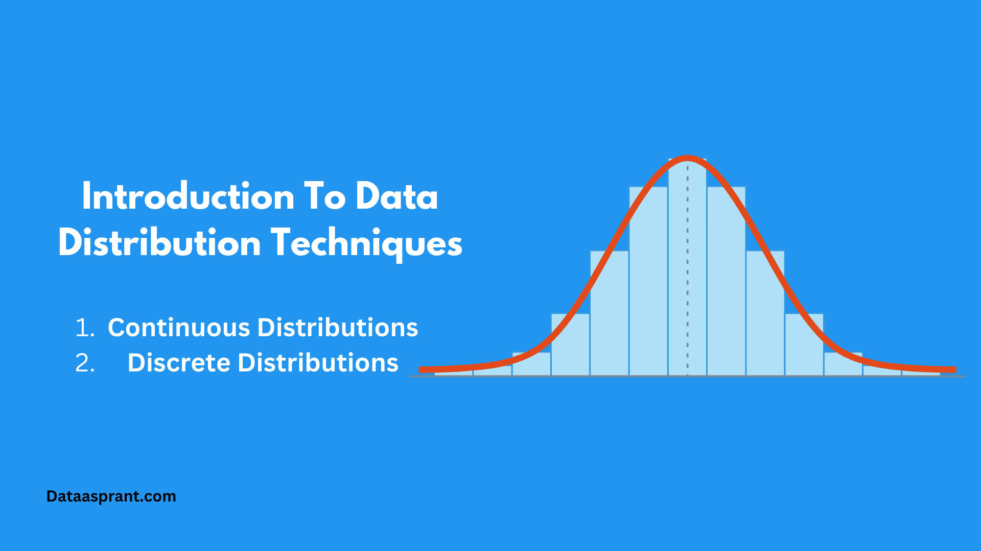
Data distribution techniques are the cornerstone of statistics and data analysis. They provide a way to describe a dataset's overall shape and behaviour, which is crucial for making informed decisions based on the data. Understanding data distributions allows you to:



- Identify patterns and trends in the data.
- Make predictions and conclude the population from which the data is drawn.
- Evaluate the reliability of your findings by accounting for variability in the data.
- Choose appropriate statistical tests and models that fit the distribution of your data.
In short, a solid grasp of data distributions will enable you to make the most of your data and draw meaningful insights.
Data distribution is a mathematical function that describes the probability of different outcomes or values in a dataset. In other words, it tells us how the data points are spread out and how likely it is to observe a particular value. There are two main types of data distributions:
- Continuous Distributions: These describe the probabilities of all possible values within a continuous range, such as height, weight, or temperature. In a continuous distribution, there's a probability associated with every point on the number line within the given range.
- Discrete Distributions: describe the probabilities of distinct, separate values, such as the number of heads when flipping a coin or the number of items sold in a store. In a discrete distribution, the probability is associated with each distinct value, and the values are typically integers.
How to Learn Data Distribution Techniques to Improve Your Data Analysis Skills
Mastering data distribution techniques will give you a strong foundation to build on as you tackle more advanced data analysis tasks. Here's how understanding data distributions can enhance your skills:
- Improved Visualization: Knowing the appropriate type of distribution for your data will help you create more accurate and informative visualisations, such as histograms or box plots.
- Better Model Selection: Understanding the distribution of your data allows you to choose the most appropriate statistical models and tests, increasing the validity and reliability of your findings.
- Accurate Predictions: When you know the underlying distribution of your data, you can make more accurate predictions about future outcomes, which is essential in fields like finance, marketing, and scientific research.
- Enhanced Problem-Solving: With a strong foundation in data distribution, you'll be better equipped to tackle complex data analysis problems and uncover hidden insights.
- Increased Credibility: Demonstrating a deep understanding of data distributions will make your analysis more convincing and credible to your audience, whether they are colleagues, clients, or stakeholders.
Now that you understand the importance of data distributions and how they can enhance your data analysis skills, let's dive deeper into the different types of distributions and how to work with them.
Basics of Data Distribution Techniques
Let's dive into the essential concepts you'll need to understand data distributions. We'll cover the two main types of distributions—continuous and discrete—and the parameters that help us describe them.
Don't worry if you're new to statistics; we'll break everything down in an easy-to-understand manner.
Definition and Types of Data Distributions
Data distribution is a mathematical function that describes how the values in a dataset are spread out and how likely it is to observe a particular value. As we discussed before there are two main types of data distributions:
Continuous Distributions:
These distributions describe the probabilities of all possible values within a continuous range. In a continuous distribution, there's a probability associated with every point on the number line within the given range.
For example, the height of people in a population can be described using a continuous distribution, as the height can take on any value within a specific range.
Discrete Distributions:
These distributions describe the probabilities of distinct, separate values. In a discrete distribution, the probability is associated with each distinct value, and the values are typically integers.
For example, the number of children in a family can be described using a discrete distribution, as it can only take on distinct whole number values (e.g., 0, 1, 2, 3, etc.).
Parameters of Data Distributions
We use various parameters to describe the shape and characteristics of a data distribution. These parameters help us summarise the data and draw insights from it. The most common parameters are:


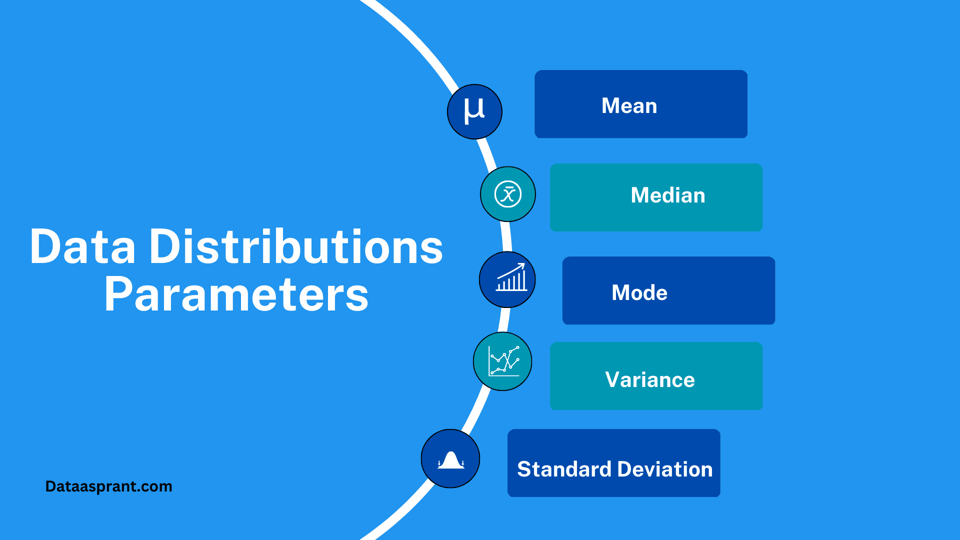

- Mean: The mean, also known as the average, is the sum of all the values in the dataset divided by the number of values. It represents the central tendency of the data and can give you an idea of the "typical" value in the dataset. However, the mean can be sensitive to extreme values or outliers.
- Median: The median is the middle value in a dataset when the values are sorted in ascending or descending order. If there's an even number of values, the median is the average of the two middle values. The median is less sensitive to extreme values than the mean, making it a better measure of the central tendency for skewed distributions.
- Mode: The mode is the value that occurs most frequently in the dataset. It's possible to have multiple modes in a dataset or even no mode at all if all values occur with equal frequency. The mode can be useful for understanding the most common outcome in a dataset, particularly in discrete distributions.
- Variance: Variance measures the dispersion or spread of the values in a dataset. It's calculated by taking the average of the squared differences between each value and the mean. A higher variance indicates a greater spread of values, while a lower variance suggests the values are more tightly clustered around the mean.
- Standard Deviation: The standard deviation is the square root of the variance. It's a measure of dispersion that is expressed in the same units as the data, making it easier to interpret than variance. A higher standard deviation indicates a larger spread of values, while a lower standard deviation indicates that the values are more closely grouped around the mean.
Common Data Distributions Types
Now that we've covered the basics of data distributions and their parameters let's explore some of the most common distributions you'll encounter in statistics. We'll explain the characteristics and applications of each distribution in a way that's easy for beginners to understand.


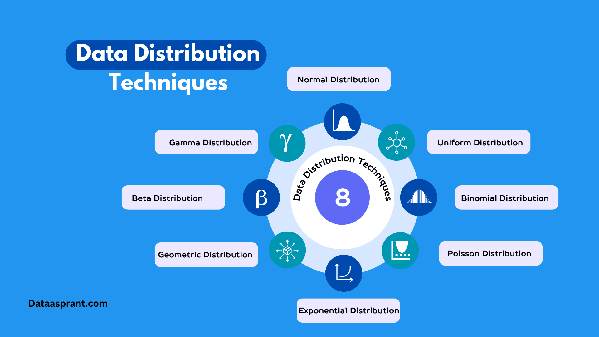

Normal Distribution (Gaussian Distribution)
Characteristics:
The normal distribution, also known as the Gaussian distribution or bell curve, is a continuous distribution characterised by its symmetrical, bell-shaped curve.
The curve is centred around the mean (µ) and is defined by its standard deviation (σ). Approximately 68% of the values fall within one standard deviation of the mean, 95% within two standard deviations, and 99.7% within three standard deviations.
Applications:
The normal distribution is prevalent in many natural and social phenomena, making it a vital tool in various fields. Some applications include:
- Quantifying measurement errors in scientific experiments
- Analyzing test scores or other performance metrics
- Modeling stock returns in finance
- Evaluating process control and quality assurance in manufacturing
Uniform Distribution
Characteristics:
The uniform distribution is a continuous distribution in which all values within a specified range have an equal probability of occurring.
The distribution is characterised by its minimum (a) and maximum (b) values, which define the range. The probability density function is constant, equal to 1/(b-a).
Applications:
The uniform distribution is often used in scenarios without prior knowledge or reason to favour one outcome over another. Some applications include:
- Simulating random events in computer programs or games
- Allocating resources evenly among different options
- Modeling the equal probability of drawing a specific card from a well-shuffled deck
Binomial Distribution
Characteristics:
The binomial distribution is a discrete distribution that models the number of successes in a fixed number of Bernoulli trials (independent experiments with two possible outcomes: success or failure).
The distribution is characterised by the number of trials (n) and the probability of success (p) in each trial.
Applications:
The binomial distribution is commonly used when the probability of success remains constant across trials. Some applications include:
- Analysing the number of heads in a series of coin flips
- Estimating the number of defective items in a production batch
- Modeling the number of correct answers on a multiple-choice test
Poisson Distribution
Characteristics:
The Poisson distribution is a discrete distribution that models the number of events occurring in a fixed interval of time or space, given a constant average rate of occurrence (λ).
The distribution is characterised by its single parameter, λ, which represents the average number of events in the interval.
Applications:
The Poisson distribution is widely used to model rare events or occurrences in various fields. Some applications include:
- Estimating the number of phone calls received at a call center per hour
- Modeling the number of defects in a manufactured product
- Analyzing the number of accidents at an intersection over a given period
Exponential Distribution
Characteristics:
The exponential distribution is a continuous distribution that models the time between events in a Poisson process (where events occur independently and at a constant average rate).
The distribution is characterised by its single parameter, λ, which represents the average rate of occurrence.
Applications:
The exponential distribution is commonly used to model waiting times or time-to-failure scenarios. Some applications include:
- Analysing the time between customer arrivals at a store or service centre
- Estimating the time until the failure of an electronic component or machine
- Modeling the time between natural disasters or other rare events
Geometric Distribution
Characteristics:
The geometric distribution is a discrete distribution that models the number of Bernoulli trials required to obtain the first success. The distribution is characterised by its single parameter, p, representing the probability of success in each trial.
The probability mass function of the geometric distribution is given by P(X=k) = p(1-p)^(k-1)
Where k is the number of trials.
Applications:
The geometric distribution is useful in scenarios where we're interested in the number of trials until the first success occurs. Some applications include:
- Determining the number of coin flips until the first head appears
- Estimating the number of calls a salesperson must make before making a sale
- Analyzing the number of attempts required to pass a driving test
Beta Distribution
Characteristics:
The beta distribution is a continuous distribution defined on the interval [0, 1], which makes it especially useful for modeling probabilities or proportions.
The distribution is characterised by two shape parameters, α and β, which determine the shape of the distribution curve. The beta distribution is highly flexible, allowing it to take on various shapes depending on the values of α and β.
Applications:
The beta distribution is widely used in Bayesian statistics, as it can act as a conjugate prior distribution for various likelihood functions. Some applications include:
- Modeling the probability of success in a binomial experiment when prior information is available
- Estimating the proportion of defective items in a manufacturing process
- Analyzing the conversion rates of online marketing campaigns
Gamma Distribution
Characteristics:
The gamma distribution is a continuous distribution that models the waiting time until an arbitrary number of events occur in a Poisson process.
The distribution is characterized by the shape parameter (k) and the scale parameter (θ). The gamma distribution reduces to the exponential distribution when the shape parameter equals 1.
Applications:
The gamma distribution is used in various fields to model waiting times, lifetimes, or other continuous, non-negative variables. Some applications include:
- Estimating the time until the failure of a complex system with multiple components
- Modeling the waiting time until a specified number of customers arrive at a service centre
- Analysing the lifespan of a biological population or the duration of certain diseases
By understanding these common data distributions and their characteristics, you'll be better equipped to identify the appropriate distribution for your data and apply the correct statistical techniques to analyze and interpret the data.
Visualizing Data Distributions
Visualisations can provide valuable insights into the shape and characteristics of a dataset. Here are three standard visualization techniques for exploring data distributions:


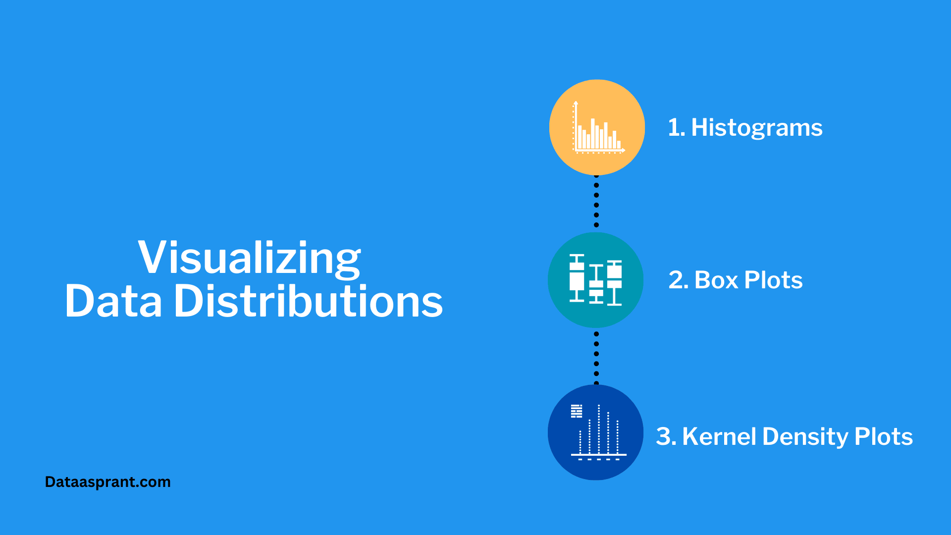

Histograms:
A histogram is a graphical representation of the distribution of a dataset. It divides the data into intervals (bins) and plots the frequency of values in each bin as a bar.
Histograms can help you identify the central tendency, dispersion, and skewness of your data and detect outliers.
Box Plots:
A box plot, also known as a box-and-whisker plot, provides a visual summary of the data by displaying the median, quartiles, and potential outliers.
The box represents the interquartile range (IQR), which contains the middle 50% of the data, while the whiskers extend to the minimum and maximum values within 1.5 times the IQR. Outliers are plotted as individual points.
Box plots can help you assess your data's symmetry, skewness, and potential outliers.
Kernel Density Plots:
A kernel density plot is a smoothed, continuous representation of a dataset's distribution. It estimates the probability density function by placing a kernel (a smooth curve) at each data point and summing the kernels.
Kernel density plots can help you visualize the shape of the distribution, identify multiple modes, and detect potential outliers.
Statistical Tests for Distribution Fitting
Once you have visually explored your data, you can use statistical tests to determine which distribution best fits your dataset. Here are three common tests for distribution fitting:


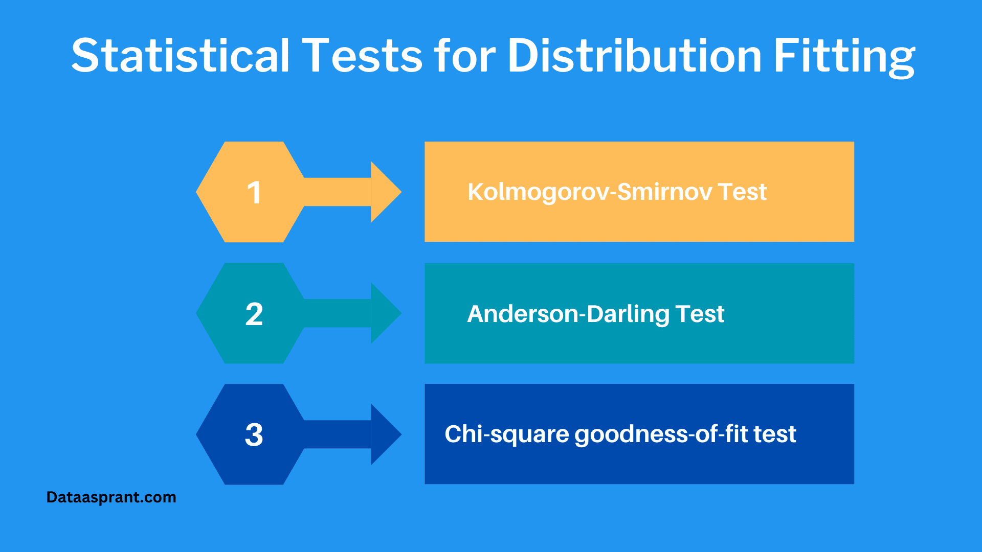

Kolmogorov-Smirnov Test:
The Kolmogorov-Smirnov (K-S) test is a non-parametric test that compares the empirical cumulative distribution function (ECDF) of your data to the cumulative distribution function (CDF) of a theoretical distribution.
The test statistic is the maximum absolute difference between the two CDFs. A small p-value (typically < 0.05) indicates that the data is inconsistent with the specified distribution.
Anderson-Darling Test:
The Anderson-Darling (A-D) test is a modification of the K-S test that gives more weight to the distribution's tails. Like the K-S test, the A-D test compares the ECDF of your data to the CDF of a theoretical distribution.
The test statistic is a weighted sum of the squared differences between the two CDFs. A small p-value indicates that the data is inconsistent with the specified distribution.
Chi-square goodness-of-fit test:
The chi-square goodness-of-fit test is a parametric test that compares the observed frequencies in your data to the expected frequencies under a specified distribution.
The test statistic is the sum of the squared differences between the observed and expected frequencies divided by the expected frequencies. A small p-value indicates that the data is inconsistent with the specified distribution.
By using visualizations and statistical tests, you can identify the distribution of your real-world data and select the appropriate models and techniques for your analysis. This process is critical for ensuring the validity and reliability of your findings.
Transforming Data Distributions
This section will discuss data transformations, their importance, and common techniques used to transform data distributions.
Understanding how to transform data can help you meet the assumptions of various statistical models and improve the interpretability of your results.


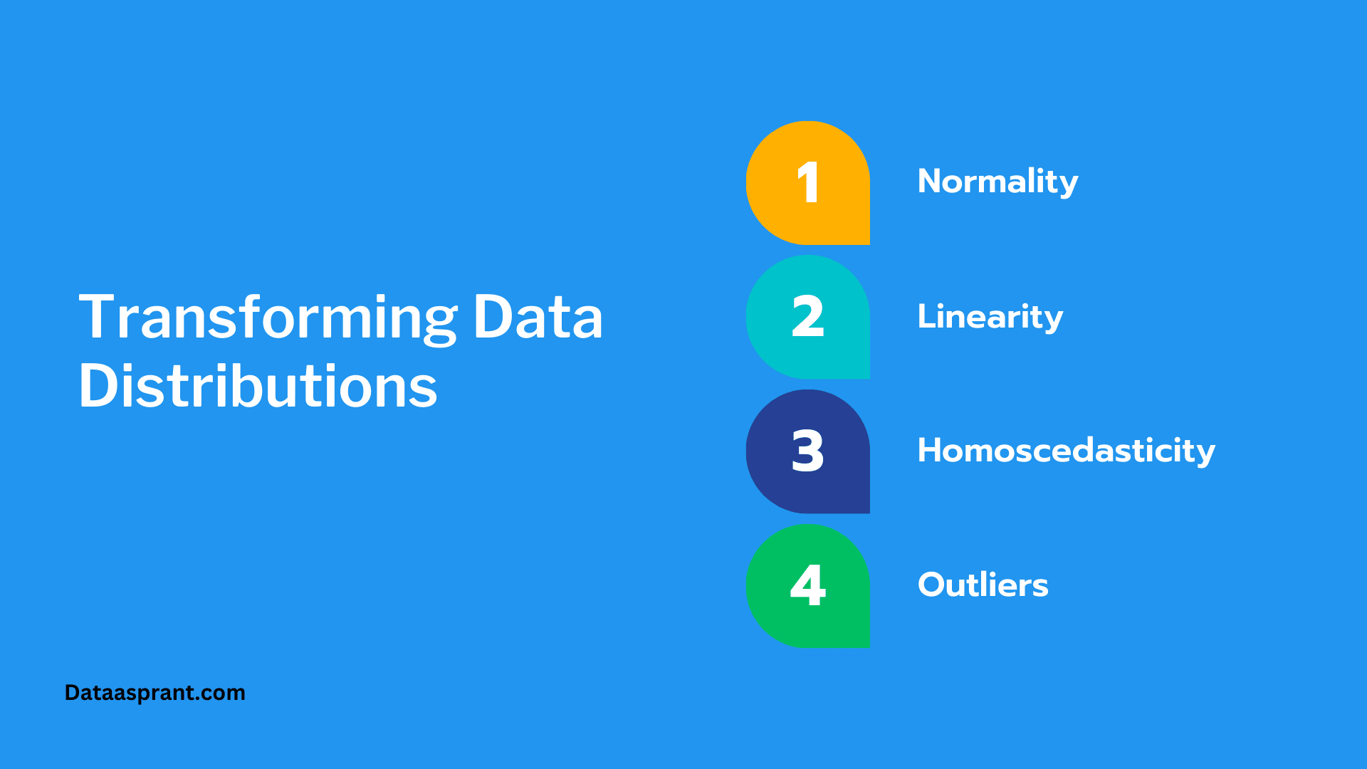

Data transformations are important for several reasons:
- Normality: Many statistical tests and models assume that the data follows a normal distribution. Transforming non-normal data can help satisfy this assumption and ensure the validity of your analysis.
- Linearity: Linear relationships are easier to model and interpret than non-linear relationships. Transformations can be used to linearize relationships between variables, making applying and interpreting linear regression models easier.
- Homoscedasticity: Statistical models often assume that the variance of the errors is constant across all levels of the predictor variables (homoscedasticity). Transformations can help stabilize the variance and improve model performance.
- Outliers: Transformations can reduce the influence of outliers and make the data more robust to extreme values.
Common Data Transformation Techniques
Here are three common data transformation techniques that can help address the issues mentioned above:
- Logarithmic Transformation: The logarithmic transformation is useful for reducing the impact of outliers, stabilizing variance, and transforming data that follows a power-law or exponential distribution. To apply a logarithmic transformation, simply take each data point's natural logarithm (log base e) or the common logarithm (log base 10). Note that this transformation can only be applied to positive values.
- Square Root Transformation: The square root transformation is useful for reducing the impact of outliers and stabilizing variance, particularly in data that follows a chi-square distribution or has a positively skewed distribution. To apply a square root transformation, take the square root of each data point. This transformation can be applied to positive and zero values but not negative ones.
- Box-Cox Transformation: The Box-Cox transformation is a family of transformations that includes the logarithmic and square root transformations as special cases. The Box-Cox transformation is defined as:
y = (x^λ - 1) / λ, for λ ≠ 0
y = log(x), for λ = 0
The parameter λ can be chosen best to approximate a normal distribution for the transformed data. You can use software or statistical packages to find the optimal value of λ based on your data.
By understanding the importance of data transformations and learning to apply common transformation techniques, you can improve the quality of your data analysis and ensure that your statistical models and tests are valid and reliable.
Using Data Distribution Techniques In Data Analysis
Understanding data distributions is crucial for various data analysis applications. This section will discuss how knowledge of data distributions can be applied to hypothesis testing, confidence intervals, regression analysis, anomaly detection, and Monte Carlo simulations.


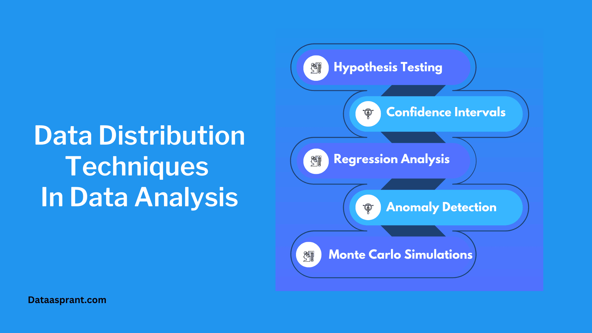

Hypothesis Testing
Hypothesis testing is a statistical method used to evaluate the validity of a claim or assumption about a population based on a sample of data. Data distributions are vital in hypothesis testing, as they are used to calculate test statistics and p-values.
Different tests are based on different underlying distributions, such as the normal distribution for t-tests or the F-distribution for analysis of variance (ANOVA). Understanding each test's assumptions and appropriate distributions is crucial for drawing accurate conclusions.
Confidence Intervals
Confidence intervals provide a range of values within which a population parameter, such as the mean or proportion, will likely fall with a certain confidence level. Data distributions are used to calculate confidence intervals, as the interval's width depends on the data's standard deviation or standard error and the chosen confidence level.
For example, a 95% confidence interval for the population mean is calculated using the sample mean, standard deviation, and the critical value from the t-distribution or the normal distribution, depending on the sample size and the underlying assumptions.
Regression Analysis
Regression analysis is a statistical technique used to model the relationship between a dependent variable and one or more independent variables.
Data distributions are essential in regression analysis, as they help to determine the appropriate model to use (linear regression, logistic regression, Poisson regression, etc.) and to assess the validity of the model assumptions such as
- Normality,
- Homoscedasticity,
- Independence of errors.
Transformations and other techniques can be applied to the data to meet these linear regression assumptions and improve the performance of the regression model.
Anomaly Detection
Anomaly detection is the process of identifying unusual patterns or outliers in a dataset that deviate significantly from the expected behaviour.
Data distributions can establish a "normal" behaviour baseline and calculate the likelihood of observing a particular data point. By comparing the observed data to the expected distribution, you can identify potential anomalies and investigate their causes.
For example, a data point that falls several standard deviations away from the mean in a normal distribution might be considered an anomaly.
Monte Carlo Simulations
Monte Carlo simulations are a computational technique used to estimate the probability distribution of an outcome by repeatedly simulating random variables and calculating the resulting statistics. Data distributions are used to generate the random variables in the simulation.
The results can be analyzed to estimate the likelihood of different outcomes or to compute confidence intervals for the estimates.
Monte Carlo simulations are widely used in finance, engineering, and other fields to model uncertainty and assess the risk of various decisions.
By understanding the role of data distributions in these data analysis applications, you can enhance your ability to perform accurate, reliable analyses and make more informed decisions based on your findings.
Tools or Libraries for Working with Data Distributions
Several software tools and libraries are available to help you work with data distributions, perform statistical analyses, and create visualizations. In this section, we will discuss popular Python libraries and R packages that are commonly used for working with data distributions.
Python Libraries for Performing Data Distribution Techniques
- NumPy: NumPy is a fundamental library for numerical computing in Python. It supports working with arrays and matrices and mathematical functions for performing statistical calculations, such as mean, median, variance, and standard deviation.
- SciPy: SciPy is a library built on top of NumPy that provides additional functionality for scientific computing, including optimization, linear algebra, and statistical functions. SciPy includes various probability distributions and statistical tests, making it a powerful tool for working with data distributions.
- Pandas: Pandas is a data manipulation library for Python that provides data structures like DataFrame and Series, which are essential for working with structured data. Pandas easily import, clean, and transform data and perform descriptive statistics and basic visualizations.
- Matplotlib: Matplotlib is a widely-used Python library for creating static, animated, and interactive visualizations. It provides various plotting functions for creating histograms, box plots, and other visualizations to explore data distributions.
- Seaborn: Seaborn is a statistical data visualization library based on matplotlib that simplifies the process of creating informative and attractive plots. Seaborn provides built-in functions for creating kernel density plots, violin plots, and other distribution visualizations and functions for exploring relationships between variables.
R Packages for Performing Data Distribution Techniques
- ggplot2: ggplot2 is a powerful and flexible R package for creating high-quality graphics using a declarative syntax. With ggplot2, you can create histograms, box plots, density plots, and other visualizations to explore data distributions and relationships between variables.
- dplyr: dplyr is a popular R package for data manipulation that provides a consistent set of verbs for working with data frames. It makes it easy to clean, transform, and summarize data and perform various statistical calculations.
- stats: The stats package is a built-in R package that provides a wide range of statistical functions, including probability distributions, statistical tests, and descriptive statistics. It is an essential tool for working with data distributions and performing various statistical analyses.
- MASS: The MASS package (Modern Applied Statistics with S) is an R package that provides functions for performing various statistical techniques, including linear and generalized linear models, clustering, and robust statistical methods. It also includes several datasets and utility functions for working with data distributions.
- fitdistrplus: fitdistrplus is an R package that simplifies the process of fitting distributions to data. It provides functions for estimating distribution parameters, assessing the goodness-of-fit, and comparing candidate distributions using various statistical tests, such as the Kolmogorov-Smirnov and Anderson-Darling tests.
By familiarising yourself with these tools and libraries, you can more efficiently work with data distributions, perform statistical analyses, and create informative visualizations to understand your data better and draw meaningful conclusions.
Conclusion
Throughout this blog post, we have covered the following key points related to data distribution techniques:
- Importance of understanding data distributions and how mastering them can enhance your data analysis skills.
- Basics of data distributions, including their definition, types, and various parameters.
- Common data distributions, such as normal, uniform, binomial, Poisson, and exponential distributions, along with their characteristics and applications.
- Identifying data distributions in real-world data using visualisation techniques and statistical tests.
- Transforming data distributions to meet the assumptions of statistical models and improve interpretability.
- Applications of data distributions in data analysis, including hypothesis testing, confidence intervals, regression analysis, anomaly detection, and Monte Carlo simulations.
- Tools and libraries for working with data distributions, including popular Python libraries and R packages.
As a newcomer to statistics, you have taken the first step in understanding the world of data distributions and their importance in data analysis. We encourage you to continue exploring different types of distributions, learn more about their properties, and apply these concepts in real-world situations.
Practice using the tools and libraries discussed in this post to become more comfortable with analysing and visualising data distributions.
Recommended Courses


Basic Statistics Course
Rating: 4.5/5




Bayesian Statistics Course
Rating: 4/5



Inferential Statistics Course
Rating: 4/5


